Python Programming for Applied Projects
Data Manipulation
Meet Pandas
So far, you've learned to handle Python's built-in data structures like lists and dictionaries. They're great, but for serious data work, you'll want something more powerful. Enter Pandas, the most popular Python library for data manipulation and analysis.
The core of Pandas is the DataFrame. Think of a DataFrame as a smart spreadsheet or a SQL table, but inside your Python code. It's a two-dimensional grid with rows and columns, where each column can have a different data type (numbers, text, dates, etc.). This structure makes it incredibly easy to organize, select, and work with your data.
Here, you will learn data manipulation and cleaning techniques using the popular python pandas data science library and introduce the abstraction of the DataFrame as the central data structure for data analysis.
To start using Pandas, you first need to import it. The community standard is to import it with the alias pd.
import pandas as pd

# Create a DataFrame from a dictionary
data = {
    'Name': ['Alice', 'Bob', 'Charlie'],
    'Age': [25, 30, 35],
    'City': ['New York', 'Los Angeles', 'Chicago']
}

df = pd.DataFrame(data)

print(df)
Running this code creates and prints a neatly formatted table. This DataFrame object, which we've called df, is what you'll use for all subsequent operations.
Getting Data In and Out
Creating DataFrames by hand is fine for small examples, but in the real world, your data will live in files. The most common format is the comma-separated values (CSV) file. Pandas makes reading these files a breeze.
Let's say you have a file named
employees.csv. Reading it into a DataFrame is a one-line command.
# Assuming 'employees.csv' is in the same directory
employees_df = pd.read_csv('employees.csv')

# Display the first 5 rows to check if it loaded correctly
print(employees_df.head())
The .head() method is a quick way to peek at your data without printing the entire table, which could be millions of rows long.
After you've manipulated your data, you'll often want to save your work. Writing a DataFrame back to a CSV file is just as simple.
# Save the DataFrame to a new file
# index=False prevents Pandas from writing the row index to the file
employees_df.to_csv('updated_employees.csv', index=False)
Besides CSVs, Pandas can handle many other file formats, including Excel spreadsheets, JSON files, and SQL databases.
Cleaning and Preprocessing
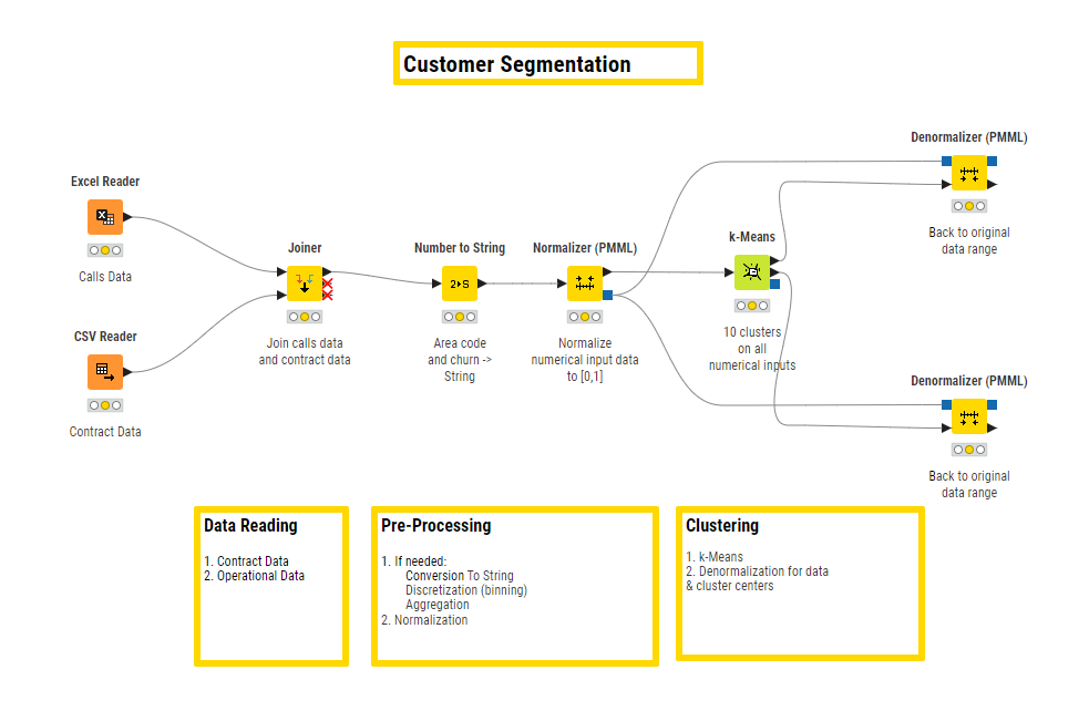
Real-world data is rarely perfect. It's often messy, with missing values, typos, or incorrect data types. A huge part of data analysis is cleaning this data to make it usable. This is often called preprocessing or data wrangling.
A common problem is missing data, which Pandas represents with NaN (Not a Number). First, you'll want to see how many missing values you have in each column.
# Count missing values in each column
print(employees_df.isnull().sum())
Once you know where the missing values are, you have two main options: drop them or fill them.
- Drop them: If you have very few rows with missing data, you might just remove them entirely.
# Drop rows with any missing values
clean_df = employees_df.dropna()
- Fill them: Sometimes, you can't afford to lose data. You might fill missing values with a placeholder, like 0, or with a calculated value, like the mean of the column.
# Fill missing ages with the average age
average_age = employees_df['Age'].mean()
employees_df['Age'].fillna(average_age, inplace=True)
Another common task is correcting data types. For example, a column of numbers might be accidentally read as text. You can fix this with the .astype() method.
# Convert the 'Salary' column from text to a number
df['Salary'] = df['Salary'].astype(float)
Basic Data Analysis
With clean data, you can start asking questions. Pandas provides powerful tools for selecting, filtering, and summarizing your data.
First, you can easily select a single column, which returns a Pandas Series (a one-dimensional array).
# Select the 'Name' column
names = df['Name']

# Select multiple columns
subset = df[['Name', 'City']]
Often, you'll want to filter your data based on a condition. For instance, let's find all employees older than 30.
# Filter for rows where Age is greater than 30
older_employees = df[df['Age'] > 30]

print(older_employees)
This technique is called boolean indexing, and it's a fast and efficient way to get subsets of your data. You can also combine multiple conditions using & (and) and | (or).
Finally, Pandas has built-in methods for getting quick summaries of your data. The .describe() method gives you a statistical summary of all numerical columns, including the mean, standard deviation, and minimum/maximum values.
# Get a statistical summary of the DataFrame
print(df.describe())
These are just the first steps. You now have the fundamental skills to load, clean, and perform basic explorations of datasets using Python and Pandas.
What is the primary, two-dimensional data structure in the Pandas library used for data manipulation and analysis?
What is the conventional and community-standard way to import the Pandas library in Python?