Linear Algebra for Quantum Physics
Linear Transformations
Rules for Moving Vectors
In the last section, we explored vector spaces, which are like playgrounds for vectors. Now, let's introduce functions that operate within these playgrounds. A linear transformation is a special kind of function that maps vectors from one vector space to another. Think of it as a rule that moves vectors around, but in a very orderly way.
A linear transformation takes a vector as an input and produces another vector as an output, all while preserving the underlying structure of the vector space.
What does “preserving the structure” mean? It means the transformation follows two fundamental rules. For any vectors and in a vector space and any scalar , a transformation is linear if:
The first rule, additivity, says that if you add two vectors and then transform the result, you get the same answer as if you transformed each vector first and then added them.
The second rule, homogeneity, says that scaling a vector and then transforming it is the same as transforming the vector first and then scaling it. These two properties ensure that grid lines in the original space remain parallel and evenly spaced after the transformation. The origin also stays put.
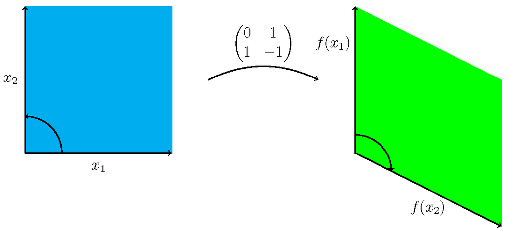
Transformations as Matrices
While the definition of a linear transformation is abstract, we can represent it using something very concrete: a matrix. For any linear transformation, there's a corresponding matrix that performs the same operation through matrix-vector multiplication. This is incredibly powerful because it turns the abstract idea of a transformation into something we can compute with.
A linear transformation is a function between vector spaces that preserves the operations of vector addition and scalar multiplication.
So, how do we find this matrix? The trick is to see what the transformation does to the basis vectors of the input space. As we learned previously, any vector can be written as a linear combination of basis vectors. If we know where the basis vectors land, we can figure out where any other vector goes.
Let's consider a transformation in a 2D space, . The standard basis vectors are and . Suppose the transformation maps them as follows:
The matrix representation of is formed by simply using these resulting vectors as its columns. We'll call this matrix .
Now, to transform any vector , we just multiply it by matrix . This works because , and by the rules of linearity, .
This direct link between transformations and matrices is a cornerstone of linear algebra. It allows us to describe complex geometric operations like rotations, shears, and scaling with simple matrix arithmetic.
Kernel and Image
Linear transformations give us a way to analyze the relationship between two vector spaces. Two key concepts that help us do this are the kernel and the image of a transformation.
kernel
noun
The set of all vectors in the input space that are mapped to the zero vector in the output space.
The kernel (also called the null space) tells us what information is lost by the transformation. If a transformation squishes a 2D plane onto a 1D line, the kernel is the line of vectors that get mapped to the origin. For a transformation , the kernel is denoted as .
image
noun
The set of all possible output vectors in the output space. It's the space that the input vectors 'land on' after the transformation.
The image (also called the range) shows us what the transformation can produce. It’s the span of the transformed basis vectors. For the same transformation , the image is denoted as .
The kernel and image are not just random sets of vectors; they are subspaces of their respective vector spaces. The dimension of the kernel is called the nullity, and the dimension of the image is called the rank. These concepts are crucial for understanding the behavior of quantum operators, which are essentially linear transformations acting on the vector spaces of quantum states.
Which pair of properties must a function satisfy for all vectors and any scalar to be considered a linear transformation?
A linear transformation maps the standard basis vectors as follows: and . What is the matrix representation of ?
Linear transformations are the verbs of linear algebra. They describe actions and relationships, turning static vector spaces into dynamic systems. By representing them with matrices, we gain a powerful tool for computation, which is essential as we move toward understanding the operations in quantum mechanics.