In system analysis, we often need to determine the output of a system given a certain input. For Linear Time-Invariant (LTI) systems, this relationship is described by an operation called convolution. In the time domain, the output signal, y(t), is the convolution of the input signal, x(t), with the system's impulse response, h(t).

Mathematically, convolution is an integral that expresses the amount of overlap of one function as it is shifted over another. It's defined as:

While direct calculation of this integral can be tedious, the Laplace transform offers a powerful shortcut. Just as the transform converted differentiation into multiplication, it simplifies convolution in the same way. The Convolution Theorem states that convolution in the time domain corresponds to simple pointwise multiplication in the s-domain.

This leads to a fundamental concept in control systems: the transfer function. The Laplace transform of the impulse response, H(s), is called the transfer function. It relates the output Y(s) to the input X(s) algebraically.

After performing analysis in the s-domain, we need a way to return to the time domain. This process is called the Inverse Laplace Transform. For simple functions, we can use tables or partial fraction expansion. However, for functions with complex poles or other intricate structures, we need a more robust method.

The formal definition of the inverse transform is given by the Bromwich integral, a contour integral in the complex plane.

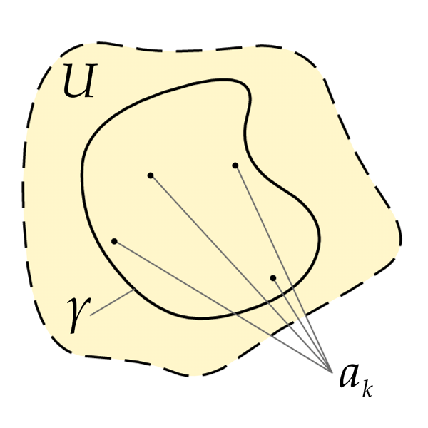
Evaluating this integral directly is difficult. Fortunately, we can use a powerful tool from complex analysis called the Residue Theorem. This theorem relates a contour integral to the properties of the function at its poles, which are points where the function becomes infinite.

To apply the Residue Theorem, we modify the Bromwich contour. We close the vertical integration path with a large semicircular arc. For t > 0, we close the contour in the left-half of the complex plane. As the radius of this arc approaches infinity, the integral along the arc typically vanishes, a condition satisfied by most functions encountered in practice.

The Residue Theorem states that the integral over this closed path is equal to 2\pi i times the sum of the residues of the function F(s)e^{st} at all the poles enclosed by the contour. Since the integral over the arc is zero, the original Bromwich integral simplifies to this sum.

This powerful method allows us to find the inverse transform for functions where simple partial fraction expansion would be difficult or impossible, especially when dealing with complex conjugate poles, which correspond to oscillatory behavior in the time domain.

By mastering this technique, we can move from any system's s-domain representation, no matter how complex, back to its physical, time-domain behavior.