Cost-Complexity Tree Pruning Deep-Dive
Comparative Implementation
Pruning in Practice With Scikit-learn
So far, we’ve covered the theory behind Cost-Complexity Pruning, from the math of the weakest link to the logic of cross-validation. Now, let's translate that theory into code. Fortunately, you don't have to manually calculate the effective alpha, , for every node. Libraries like Scikit-learn have built-in functions that handle the heavy lifting.
The key method is cost_complexity_pruning_path, available on Scikit-learn's decision tree classifiers. When you train a decision tree, you can call this method to get the sequence of alpha values that mark each pruning step. The function returns a dictionary-like object containing two key arrays: ccp_alphas and impurities.
The
ccp_alphasarray contains the series of effective alpha values. Each value represents the exact threshold where a new node (the current weakest link) gets pruned. Theimpuritiesarray shows the total impurity of the leaves for each corresponding tree in the pruning sequence.
With these alphas, we can generate the entire sequence of pruned trees. We simply loop through the ccp_alphas and train a new DecisionTreeClassifier for each one, setting the ccp_alpha parameter to the current value in the loop. This creates a collection of models, each one slightly less complex than the last. The final alpha value results in a tree with only the root node.
# Assume X_train and y_train are your training data
from sklearn.tree import DecisionTreeClassifier

# First, train a full, unpruned tree
clf = DecisionTreeClassifier(random_state=0)
clf.fit(X_train, y_train)

# Get the pruning path
path = clf.cost_complexity_pruning_path(X_train, y_train)
ccp_alphas, impurities = path.ccp_alphas, path.impurities

# Create a list to store one tree for each alpha
clfs = []
for ccp_alpha in ccp_alphas:
    # Prune the tree using the ccp_alpha parameter
    clf_pruned = DecisionTreeClassifier(random_state=0, ccp_alpha=ccp_alpha)
    clf_pruned.fit(X_train, y_train)
    clfs.append(clf_pruned)

# The last model in clfs is the root-only stump
print(f"Number of nodes in the last tree: {clfs[-1].tree_.node_count}")
This process gives us a series of candidate trees. By plotting the number of nodes or tree depth against the ccp_alpha, you can visualize the trade-off. As alpha increases, the tree's complexity shrinks. Now the only question is: which tree is the best? As you'll recall, we use to find out. We calculate the accuracy of each pruned tree on a validation set and pick the alpha that gives the best performance.
A Tale of Two Libraries
Scikit-learn isn't the only tool for the job. In the R programming language, the popular rpart package offers a similar mechanism. However, instead of alpha, rpart uses a parameter called cp, which stands for complexity parameter. While the naming is different, the concept is identical.
cp in rpart serves the same function as ccp_alpha in Scikit-learn: it's the value that the improvement from any split must exceed for it to be attempted. By setting a cp value, you are effectively setting a minimum alpha for the tree. The rpart library provides a table of cp values that correspond to different tree sizes, allowing you to select the one that performs best under cross-validation.
| Library | Parameter Name | What it Represents |
|---|---|---|
| Scikit-learn | ccp_alpha | The complexity penalty applied to the number of leaves. |
R (rpart) | cp | A threshold for improvement; analogous to . Any split that does not decrease the overall lack of fit by a factor of cp is pruned. |
Pruning vs. Forests
This brings us to an interesting comparison. Cost-Complexity Pruning focuses on taking one, potentially overgrown tree and simplifying it to improve generalization. A takes a different approach. Instead of building one carefully tuned model, it builds an entire 'forest' of simple, decorrelated decision trees and aggregates their predictions.
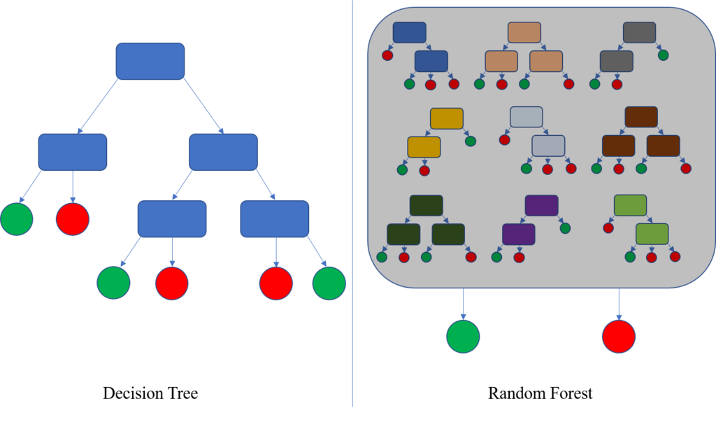
Each tree in a Random Forest is intentionally weak. It's typically trained on a random subset of the data and considers only a random subset of features at each split. This process creates a diverse set of models. While any single tree might be inaccurate, the collective wisdom of the forest is often highly accurate and robust against overfitting.
Pruning a single tree gives you one simple, interpretable model. A Random Forest gives you a high-performance 'black box' model composed of many simple parts. Neither approach is universally better; the choice depends on whether you prioritize interpretability or predictive power.
In Scikit-learn, which method is called on a trained decision tree classifier to get the sequence of alpha values for pruning?
After generating a list of ccp_alphas, what is the next step in the Cost-Complexity Pruning process to find the optimal tree?