Cost-Complexity Tree Pruning Deep-Dive
Pruning Objectives
The Problem with Perfect Trees
When you grow a decision tree, it's tempting to let it branch out until every single data point in your training set is perfectly classified. This creates a 'maximal tree'—a complex, sprawling structure that has learned the training data inside and out. The problem? This tree has likely learned not just the underlying patterns, but also the noise and random quirks specific to that one dataset.
This phenomenon is called A model that overfits is like a student who memorizes the answers to a practice test but doesn't understand the concepts. When faced with new questions, the student falters. Similarly, an overfit decision tree performs poorly on new, unseen data because it's too tailored to its training examples.
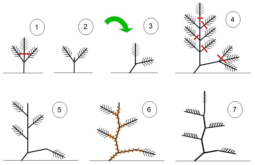
Pruning is a method used to cut a decision tree's size by eliminating parts that have minimal ability in target variable prediction.
To prevent this, we need to prune the tree. Think of it like pruning a bonsai tree. You snip away branches that aren't contributing to the overall desired shape, resulting in a healthier, more elegant tree. In our case, we want to snip away branches that capture noise instead of signal.
Cost-Complexity Pruning
But how do we decide which branches to cut? We need a formal way to measure the trade-off between a tree's simplicity and its accuracy. This is where cost-complexity pruning, also known as weakest link pruning, comes in. The goal is to find the subtree that best balances these two competing factors.
We use a function called the cost-complexity measure to guide us. It introduces a penalty for having too many leaves.
The parameter is the key. When , there is no penalty for complexity, and the best tree is simply the largest, most complex one. As we increase , the cost of having extra leaves becomes higher, forcing the algorithm to favor smaller trees. The process generates a sequence of subtrees, each being the optimal tree for a certain range of . We then use a separate validation dataset to choose the best subtree from this sequence—the one that generalizes best.
Balancing Bias and Variance
This pruning process is a direct application of the A core concept in machine learning, it describes the delicate balance between two types of error.
A large, unpruned tree has low bias but high variance. It fits the training data perfectly but is unstable and sensitive to small changes. A small, heavily pruned tree (or even just a stump) has high bias but low variance. It's stable but too simple to capture the important relationships in the data.
Cost-complexity pruning allows us to navigate this tradeoff systematically, finding a tree that strikes a good balance and is most likely to perform well on data it hasn't seen before.
Now, let's test your understanding of these concepts.
What is the primary problem with growing a decision tree until it perfectly classifies every point in the training data, creating a 'maximal tree'?
In cost-complexity pruning, what is the role of the complexity parameter, ?