The Khintchine inequality provides a powerful way to understand the size of sums of random variables. Specifically, it gives us upper and lower bounds for the expected value of a weighted sum of Rademacher random variables. As a quick refresher, a Rademacher random variable is a simple type of variable that takes the value +1 or -1, each with a probability of 1/2.

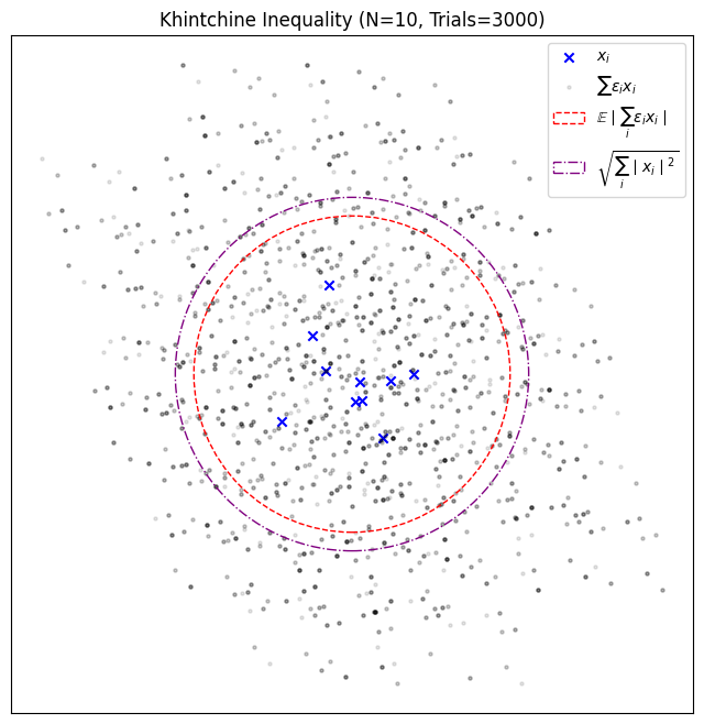
Imagine you have a series of these random coin flips, let's call them $\epsilon_1, \epsilon_2, \dots, \epsilon_n$. Now, you assign a weight, $a_k$, to each flip. The Khintchine inequality helps us predict the likely magnitude of the final sum, $S = \sum_{k=1}^n a_k \epsilon_k$. It connects the expected size of this random sum to the simple sum of the squares of the weights.

In essence, the inequality states that the average size of the random sum is proportional to the square root of the sum of the squares of the weights. The constants $A_p$ and $B_p$ ensure the relationship holds for any moment $p$ you choose. This is a remarkable result because it links a probabilistic quantity (the expectation of a random sum) to a deterministic one (the norm of the coefficients).

The Khintchine inequality is more than just a theoretical curiosity. It has significant applications in several fields.

In functional analysis, a branch of pure mathematics, it's used to compare different ways of measuring the "size" of functions or vectors in infinite-dimensional spaces. It shows that certain norms, which might look very different, are actually equivalent.

In computer science and information theory, it appears in the analysis of algorithms that use randomness. For example, in techniques like random projections (used for dimensionality reduction), the inequality helps prove that distances between data points are preserved, which is crucial for the algorithm's success.

Let's see the inequality in action with a simple case where $p=2$. We have the sum $S = \sum_{k=1}^n a_k \epsilon_k$. We want to calculate the expected value of its square, $\mathbb{E}[S^2]$.

Because expectation is linear, we can move it inside the sums.

Now, we consider two cases for the expectation $\mathbb{E}[\epsilon_i \epsilon_j]$.

1. When $i \neq j$: Since $\epsilon_i$ and $\epsilon_j$ are independent, $\mathbb{E}[\epsilon_i \epsilon_j] = \mathbb{E}[\epsilon_i] \mathbb{E}[\epsilon_j]$. The expectation of any single Rademacher variable is $1 \cdot (1/2) + (-1) \cdot (1/2) = 0$. So, the product of their expectations is $0 \cdot 0 = 0$.

2. When $i = j$: The term becomes $\mathbb{E}[\epsilon_i^2]$. Since $\epsilon_i$ is either +1 or -1, its square is always 1. Thus, $\mathbb{E}[\epsilon_i^2] = 1$.

This means the only terms that survive the double summation are those where $i=j$.

The full proof for general $p$ is more involved, but this example gives a taste of the underlying mechanics. It relies on the independence and symmetry of the Rademacher variables to cancel out most of the terms.

The Khintchine inequality is a cornerstone result, connecting the probabilistic world of random sums to the deterministic world of vector norms.