How do things grow? A colony of bacteria, the value of an investment, the spread of a new technology—they all follow patterns. Growth modeling is the practice of capturing these patterns with mathematics. It allows us to understand the forces driving change and even predict what might happen next.

At its core, a growth model is a simplified description of a real-world system. By stripping away complexity, we can focus on the key factors that influence growth. This is incredibly useful in fields like biology, where we model population dynamics; in economics, to understand market trends; and in technology, to forecast the adoption of new products.

We'll start with two of the most fundamental models of growth: exponential and logistic. They represent two classic scenarios—unlimited growth and growth with limits.

Imagine a single bacterium that divides into two every hour. After one hour, you have two. After two hours, you have four. After three, you have eight. The population doubles at a constant rate. This is exponential growth. The rate of growth is proportional to the current size of the population—the more you have, the more you get.

This creates a distinct "J" shape when plotted on a graph. It starts slow, almost flat, and then accelerates, shooting upwards dramatically. We can describe this mathematically.

Here’s what the pieces mean:

• $N(t)$ is the population size at time $t$.
• $N_0$ is the initial population size (at time $t=0$).
• $r$ is the constant growth rate.
• $e$ is Euler's number, the base of the natural logarithm (approximately 2.718).

This equation is powerful. It lets us model anything that grows at a constant percentage rate, from compound interest in a savings account to the initial spread of a virus.

But there's a catch. In the real world, growth can't continue unchecked forever. Resources are finite. Space is limited. This brings us to a more realistic model.

Most populations can't grow exponentially indefinitely. Eventually, they run into limits—not enough food, too many predators, or a lack of space. This is where logistic growth comes in. It describes growth that slows down as it approaches a limit, known as the carrying capacity.

The logistic growth curve looks like a stretched-out "S." It starts off looking exponential, with rapid acceleration. Then, as the population approaches the environment's carrying capacity, the growth rate slows, and eventually, the population size levels off.

The concept of carrying capacity, or $K$, is the maximum population size that an environment can sustain. As the population $N$ gets closer to $K$, the growth rate approaches zero. This dynamic is often expressed using a differential equation.

For logistic growth, the equation looks like this.

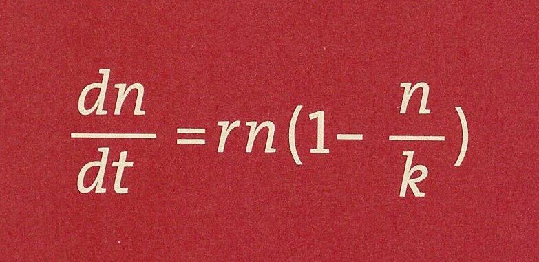
Let's break it down:

• $\frac{dN}{dt}$ represents the rate of population growth over time.
• $r$ is the maximum growth rate.
• $N$ is the current population size.
• $K$ is the carrying capacity.

The term $(1 - N/K)$ is the key. When the population $N$ is very small compared to $K$, this term is close to 1, and the growth is nearly exponential ($rN$). But as $N$ approaches $K$, the term $(1 - N/K)$ gets closer to 0, slowing growth to a halt.

These models aren't just abstract ideas; they describe the world around us.

Biology: Ecologists use logistic models to understand how animal populations are regulated by their environment. This is crucial for conservation efforts, helping to determine sustainable habitats for endangered species.

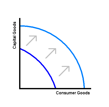
Economics: Economic growth itself can be modeled. A country's production capacity can expand over time, a concept sometimes visualized with a production possibility curve.

Technology: The adoption of new technologies often follows an S-curve. Think about smartphones. At first, only a few early adopters had them (the slow start). Then, adoption exploded (the steep part of the curve). Finally, as nearly everyone who wants one has one, the market becomes saturated, and the growth rate levels off.

Understanding these basic models provides a powerful toolkit for analyzing change. While real-world systems are often more complex, the principles of exponential and logistic growth form the foundation for understanding how things evolve over time.

Now, let's test your understanding of these fundamental concepts.