Taylor Series in Econometrics
Introduction to Taylor Series
Approximating Functions
Many functions in mathematics are complicated. Think of trigonometric functions like or the exponential function . Calculating their exact values can be tough. But what if we could approximate them using something much simpler, like a polynomial? Polynomials are friendly. They're just sums of powers of , like , and they're easy to calculate, differentiate, and integrate.
The core idea is to build a polynomial that acts just like our target function, at least around a specific point. Let's say we want to approximate a function near a point .
The simplest approximation is a constant. The best constant value to use near is simply the function's value at that point, . This is a flat horizontal line. It's not a great approximation, but it's a start.
We can do better with a line. The best line that approximates the function at is its tangent line. From basic calculus, we know the equation for the tangent line is:
Notice that this polynomial, , has the same value as at , and it also has the same first derivative. It matches the function's value and its slope at that specific point.
To get an even better fit, we can use a quadratic polynomial that also matches the function's second derivative (its concavity). If we keep matching higher and higher order derivatives, our polynomial becomes a better and better approximation of the original function near our chosen point. Extending this idea to an infinite number of terms gives us the Taylor series.
The Taylor Series Formula
A Taylor series is an infinite polynomial that represents a function. It's constructed by matching all the derivatives of the function at a single point, . The general formula for the Taylor series of a function centered at is:
Let's break that down:
- is the nth derivative of the function , evaluated at the point . For , it's just the function itself, .
- is the factorial of (e.g., ).
- is the polynomial term.
When the series is centered at , it gets a special name: the Maclaurin series. The formula is a bit simpler:
Common Expansions
Let's see this in action by finding the Maclaurin series for . We need to find its derivatives and evaluate them at . The function is . The magic of is that its derivative is always itself. So, , , and so on.
Evaluating these at , we get , , , etc. All derivatives are 1 at the origin.
Plugging these into the Maclaurin series formula gives us:
Since $0! = 1$ and $1! = 1$, this simplifies to one of the most famous series in mathematics:
Other essential functions have well-known Maclaurin series. For sine and cosine, the derivatives cycle through a pattern of four.
The Maclaurin series for includes only the odd powers of :
The Maclaurin series for includes only the even powers of :
When Does This Work?
An infinite sum doesn't always produce a finite number. For a Taylor series to be useful, it must converge. That is, as you add more and more terms, the sum must get closer and closer to the actual value of the function.
For a given function and a center point , the Taylor series might converge for all values of , for some values of , or only for . The set of values for which the series converges is called the interval of convergence. The distance from the center to the edge of this interval is the radius of convergence.
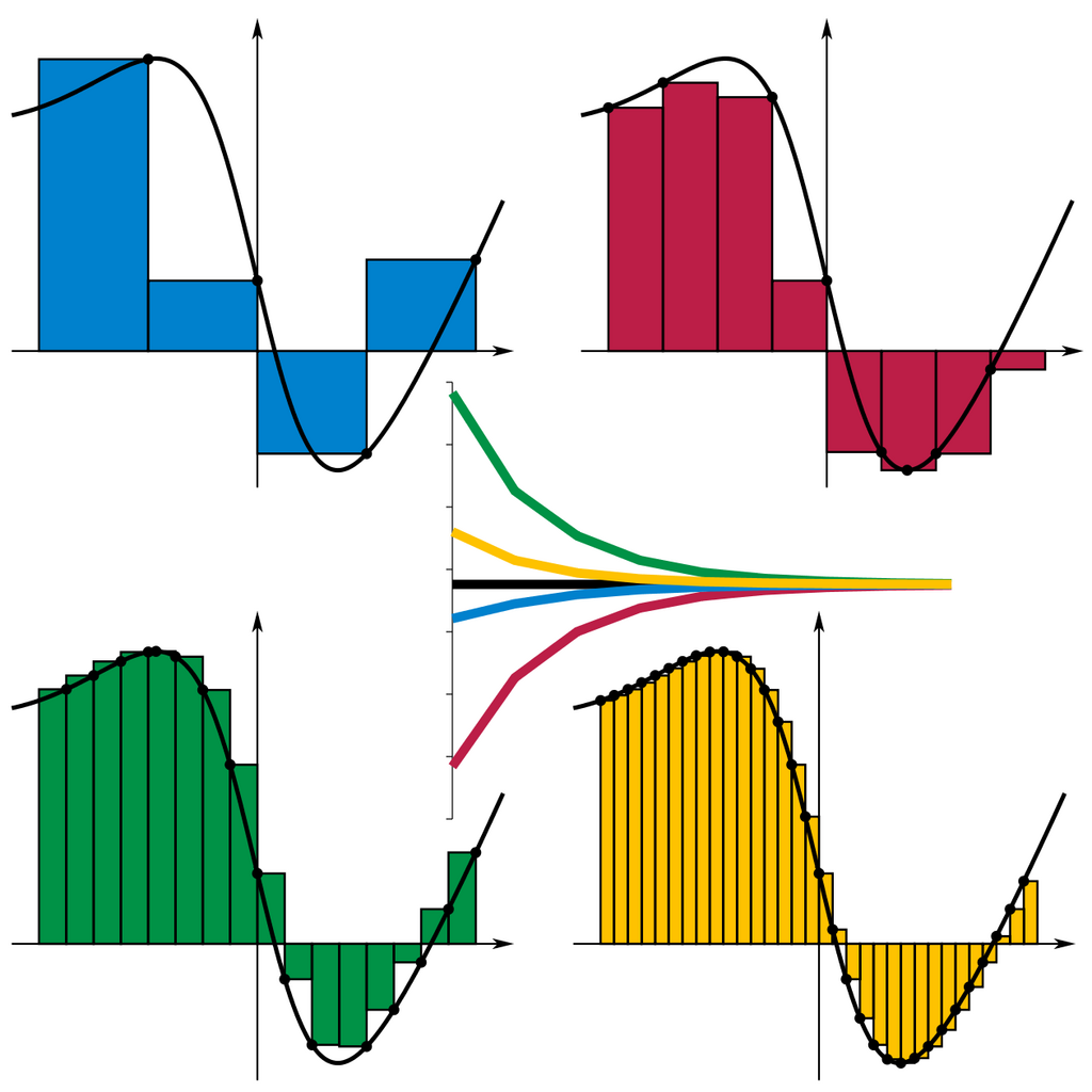
Luckily, for the common functions we just looked at (, , and ), their Maclaurin series converge for all real numbers. Their radius of convergence is infinite. This means you can use these series to approximate the functions for any value of , though you'll need more terms to get a good approximation the farther you are from the center point.
However, not all functions are so well-behaved. The series for other functions might only converge within a specific range, which is crucial to know before using the approximation.
What is the primary purpose of constructing a Taylor series for a function?
A Taylor series that is centered at the point is known by what special name?
Taylor series provide a powerful way to re-express functions as infinite polynomials, making them easier to analyze and compute.