In models like Lasso regression or gradient boosting, the focus is often on minimizing a loss function. You find the line or curve that best fits the data by reducing the error between your predictions and the actual values. Support Vector Machines (SVMs) approach classification from a different angle. Instead of just minimizing error, an SVM's primary goal is to find the most confident and robust decision boundary possible. It achieves this by maximizing the margin—the empty space between the classes.

Imagine a line drawn on a piece of paper to separate red dots from blue dots. You could draw the line so it just barely separates the two colors, skimming right past the outermost dots. Or, you could draw it right down the middle of the empty space between them. The SVM chooses the latter. This wider margin makes the model more robust to new, unseen data points. The decision boundary an SVM creates is called a hyperplane and it is the key to the whole process.

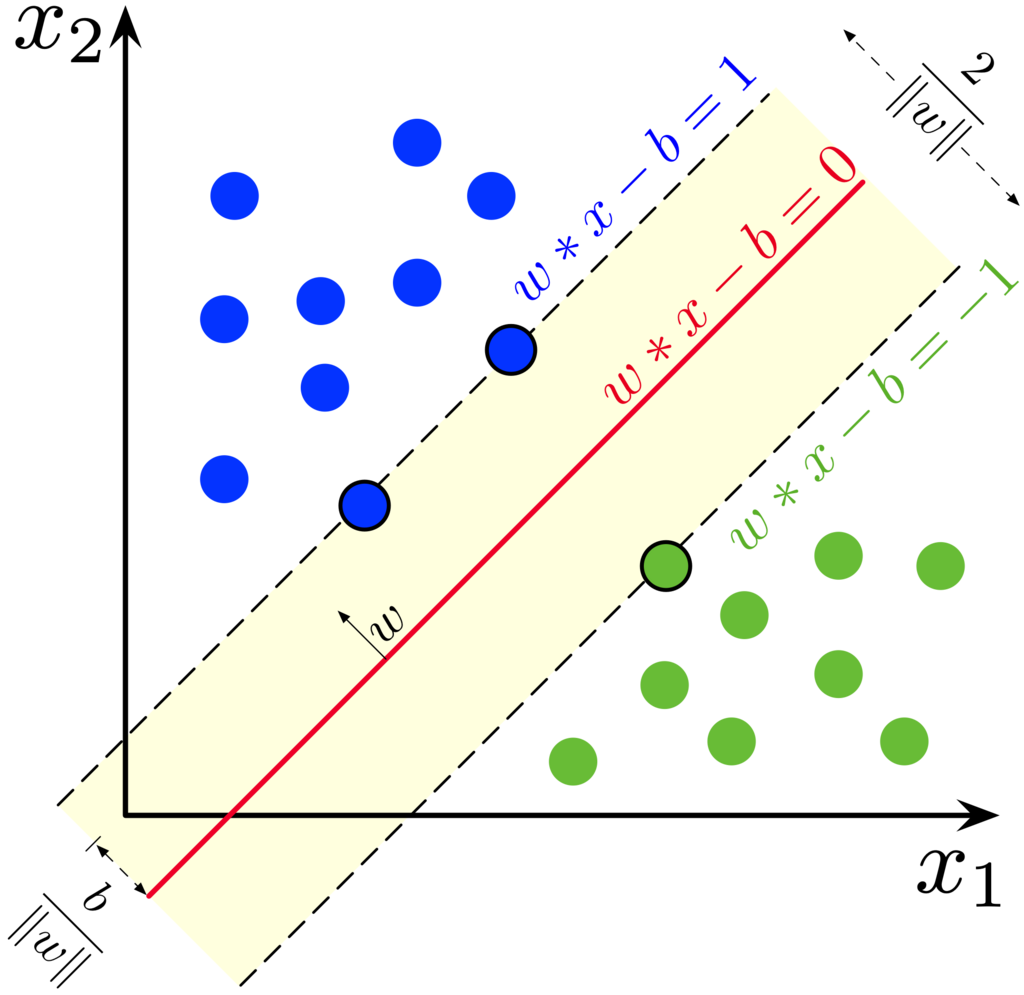
For a two-dimensional problem, the hyperplane is just a line. In three dimensions, it's a flat plane. In higher dimensions, it's a hyperplane—a subspace that is one dimension less than its surrounding space. We can define this hyperplane mathematically with a simple equation. For an input vector $x$, the equation is:

Any point $x$ that lands on the hyperplane will satisfy this equation. Points on one side will result in a positive value ($w^T x + b > 0$), and points on the other will result in a negative value ($w^T x + b < 0$). This simple classification rule forms the basis of the SVM.

So, how do we measure the margin? We start with what's called the functional margin. For a single data point $(x_i, y_i)$, where $y_i$ is the class label (+1 or -1), the functional margin is simply the raw output of our decision function, scaled by the label:

While simple, the functional margin has a flaw: we can arbitrarily increase it by scaling $w$ and $b$ (for example, by replacing them with $2w$ and $2b$) without actually changing the decision boundary itself. The line stays in the same place. To get a true, scale-invariant measure of distance, we need the geometric margin. This is the actual Euclidean distance from a point $x_i$ to the hyperplane.

The data points that lie closest to the hyperplane, right on the edge of the margin, are called support vectors They are the critical elements of the dataset, as they are the only points that determine the position and orientation of the optimal hyperplane. If you were to move any of the other data points, the hyperplane wouldn't change. But if you move a support vector, the hyperplane will shift.

Our goal is to maximize the geometric margin for the entire dataset. Let $\gamma$ be the margin for the dataset. The optimization problem can be stated as: find the $w$ and $b$ that maximize $\gamma$.

This looks a bit tricky to solve. We can simplify it. For the support vectors, the functional margin $y_i(w^T x_i + b)$ will be exactly equal to some value. We can be clever and set this value to 1. This is just a matter of scaling; we can always find a $w$ and $b$ to make it true. So for the support vectors, we have $\hat{\gamma} = 1$. This means the geometric margin is $\gamma = 1 / \|w\|$.

This insight transforms our optimization problem. For mathematical convenience (it makes the derivative cleaner), we choose to minimize $\frac{1}{2}\|w\|^2$ instead of $\|w\|$. This doesn't change the solution. Our new, much simpler problem is:

And there we have it. We've turned a geometric goal—find the widest possible street between two neighborhoods—into a well-defined quadratic optimization problem that can be solved efficiently. By minimizing the magnitude of the weight vector $w$, we find the hyperplane that is maximally confident in its classifications.

Let's review what we've covered.