Spectral Methods in CFD
Introduction to Spectral Methods
A Global Approach to Equations
Many problems in science and engineering, from predicting the weather to designing an airplane wing, boil down to solving partial differential equations (PDEs). Since finding exact, pen-and-paper solutions is often impossible, we turn to computers for numerical approximations.
A common strategy is to break the problem down. The finite difference method (FDM) approximates derivatives at a point using values from its immediate neighbors. The finite element method (FEM) divides the entire problem space into a mesh of smaller, simpler shapes, solving the equation on each little piece.
Both of these are local methods. They build a solution piece by piece, relying on information from a small surrounding area. But there's another way that takes a more holistic view.
Thinking Globally with Spectral Methods
Spectral methods operate on a different philosophy. Instead of making local approximations, they represent the solution across the entire domain as a sum of carefully chosen basis functions. These functions are global, meaning they are non-zero over the whole problem area.
Think of it like describing a complex musical chord. You could describe the pressure wave point by point (like finite differences), or you could describe it as the sum of a few pure notes—a C, an E, and a G. This is the spectral idea. The basis functions are like the pure notes, and the solution is the chord they form when combined.
The most common basis functions are trigonometric polynomials (sines and cosines), which form the basis of the Fourier series. For other problems, mathematicians use different sets of functions, like Chebyshev or Legendre polynomials, which have useful properties.
There are a few flavors of spectral methods, such as the Galerkin, Tau, and Collocation methods. They differ in how they ensure the approximate solution satisfies the PDE, but all share the core idea of using global basis functions.
The Power of Exponential Convergence
The main advantage of spectral methods is their incredible accuracy for problems with smooth solutions. This is often called "spectral accuracy."
As you increase the number of grid points (for FDM/FEM) or basis functions (for spectral methods), the error in your approximation gets smaller. This is called convergence. For FDM and FEM, the error typically decreases polynomially. For example, doubling the number of points might cut the error by a factor of four () or eight ().
For spectral methods, the error decreases exponentially. This means adding just one or two more basis functions can reduce the error by orders of magnitude. The convergence is much, much faster.
For smooth problems, spectral methods can achieve the same accuracy as local methods with far fewer degrees of freedom.
Real-World Hurdles
If spectral methods are so accurate, why aren't they used for everything? Their biggest drawback is handling complex geometries. They work best on simple domains like squares, cubes, and circles, where the basis functions fit naturally.
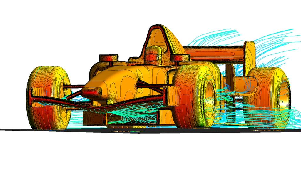
Trying to model the airflow around an intricate shape, like a race car, with a single set of global functions is extremely difficult. The rigid structure of the basis functions doesn't easily conform to irregular boundaries. This is where the flexibility of finite element methods, with their meshes of simple shapes, truly shines.
Applying boundary conditions can also be more complicated. Because each basis function spans the whole domain, enforcing a condition at one point can have ripple effects everywhere else. In local methods, adjusting a value at the boundary only directly affects its immediate neighbors.
This trade-off between accuracy and geometric flexibility is central to choosing a numerical method. Researchers have developed clever ways to combine the strengths of different approaches, such as spectral element methods, which use high-accuracy spectral techniques inside simple elements of a larger mesh.
| Method | Approach | Strengths | Weaknesses |
|---|---|---|---|
| Finite Difference | Local | Simple to implement | Struggles with complex shapes |
| Finite Element | Local | Handles complex shapes well | More complex to set up |
| Spectral | Global | Extremely high accuracy | Poor with complex shapes |
Understanding these different tools helps engineers and scientists pick the right one for the job, balancing the need for precision with the complexity of the real-world problem they're trying to solve.