Reinforcement and Continual Learning Explained
Dynamic Programming and Temporal Difference Learning
Finding the Optimal Policy
In previous sections, we learned about Markov Decision Processes (MDPs) and the Bellman equations, which give us a mathematical map of our environment and a way to evaluate how good a policy is. Now, let's explore how an agent can use this map to find the best possible route—the optimal policy.
One powerful set of tools for this task comes from Dynamic Programming (DP). DP is a classic method for solving complex problems by breaking them down into simpler, overlapping subproblems. For reinforcement learning, this means finding the optimal policy by solving the Bellman equations. A key thing to remember about DP is that it requires a perfect model of the environment. The agent must know all the state transition probabilities and rewards beforehand.
Dynamic programming methods require a complete model of the environment. They're great for planning when you know all the rules, like in a game of chess.
Policy Iteration
Policy iteration is an elegant, two-step dance an agent performs to find the optimal policy. It repeats these two steps until the policy stops improving, at which point it has found the best one.
-
Policy Evaluation: The agent starts with a random policy, . The first step is to figure out how good this policy is. It calculates the state-value function for every state by applying the Bellman equation. This is like walking through a maze with a specific set of directions and mapping out how good each spot is based on that path.
-
Policy Improvement: Once the agent knows the value of each state under the current policy, it tries to improve its directions. For each state, it looks at all possible actions and checks if taking a different action would lead to a better outcome. It greedily chooses the action that leads to the highest expected value. This creates a new, better policy, .
The agent then takes this new policy and repeats the dance: evaluate, improve, evaluate, improve. This process is guaranteed to converge to the optimal policy.
Value Iteration
Value iteration is a more streamlined approach. Instead of going through the full process of evaluating a policy completely before improving it, value iteration combines these steps. It directly calculates the optimal value function, , by repeatedly applying the Bellman optimality equation.
The algorithm initializes the value function for all states to some value (often zero). Then, in each iteration, it updates the value of each state using the values of its neighbors. It essentially asks, "What's the maximum possible value I can get from this state if I take the best possible action right now?"
This process continues until the value function converges—meaning the updates become so small they don't matter anymore. Once the optimal value function is found, the agent can easily determine the optimal policy by picking the action that maximizes the expected value for each state.
Learning Without a Map
Dynamic programming is powerful, but it has a big catch: it needs a perfect model of the environment. In the real world, agents often don't have this map. A robot exploring a new building doesn't know the exact probability of its wheels slipping on a patch of floor.
This is where model-free methods come in. These algorithms allow an agent to learn the optimal policy simply by interacting with the environment and observing outcomes. One of the most important ideas in model-free learning is Temporal Difference (TD) learning.
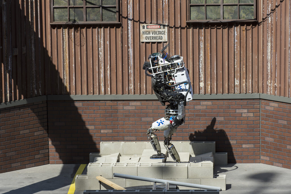
TD learning is a clever blend of ideas from dynamic programming and another model-free method called Monte Carlo. Like Monte Carlo methods, TD learning learns directly from experience. But like DP, it updates its value estimates based on other learned estimates, a technique called bootstrapping. It doesn't need to wait until the end of an episode to update its knowledge.
Imagine you're trying to predict how long your commute will take. You initially guess 30 minutes. After 10 minutes, you hit unexpected traffic and realize it's going to take at least another 30 minutes from your current spot. You don't wait until you get to work to update your belief. You immediately adjust your total estimate from 30 minutes to 40 minutes. That's the essence of TD learning.
TD learning updates its predictions on the fly, based on the difference between what it expected to happen and what actually happened.
The core of TD learning is the TD error, which measures the difference between the estimated value of a state and a more accurate estimate based on the reward received and the value of the next state. The basic update rule for the value of a state looks like this:
Here, is the learning rate, which controls how much the new information changes the current estimate. The term inside the brackets is the TD error. This simple but powerful idea is a cornerstone of modern reinforcement learning, allowing agents to learn effectively even when they don't know the rules of the game.
| Method | Requires Model? | How it Updates | Key Idea |
|---|---|---|---|
| Dynamic Programming | Yes | Uses Bellman equations | Solves the MDP with a full model. |
| TD Learning | No | Uses TD error from experience | Learns from partial information without a model. |
Now that we understand these fundamental approaches, let's test your knowledge.
What is a fundamental requirement for using Dynamic Programming (DP) methods like Policy Iteration and Value Iteration in reinforcement learning?
Which pair of repeating steps accurately describes the Policy Iteration algorithm?