At its heart, quantum computing is described using the language of linear algebra. The first concept to grasp is the vector space, which is the stage where all the action happens. Don't let the name intimidate you. Think of a simple flat plane, like a sheet of graph paper that stretches out infinitely. That's a 2D vector space.

Every vector space has a set of fundamental directions called basis vectors. These are the building blocks for every other vector in the space. For our 2D graph paper, the familiar directions along the x-axis and y-axis can serve as our basis vectors. We might label them $\hat{\imath}$ and $\hat{\jmath}$, or in quantum notation, $|0\rangle$ and $|1\rangle$.

The powerful idea here is that any vector in the space can be described as a unique mix of these basis vectors. This mix is called a linear combination. You're just taking a certain amount of one basis vector and adding it to a certain amount of the other.

If vectors represent states, we need a way to change them. This is done with linear transformations. A transformation is a rule that moves every vector in the space to a new position, but it does so in a consistent, structured way. Think of it as warping the entire sheet of graph paper. Straight lines must stay straight, and the origin (0,0) doesn't move. Common transformations include rotations, stretches, and shears.

How do we write down these transformations? With matrices. A matrix is just a grid of numbers that encodes exactly how a transformation acts on the basis vectors. If you know where the basis vectors land after a transformation, you know where every other vector will land, too. The matrix is a complete instruction manual for the transformation.

For any given linear transformation, there are often special vectors that don't change their direction. When the transformation is applied, these vectors are only stretched or shrunk, not knocked off their original line. These special vectors are called eigenvectors.

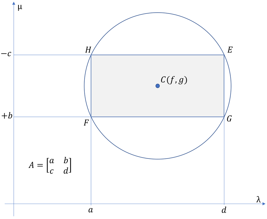
The factor by which an eigenvector is stretched or shrunk is called its eigenvalue. Each eigenvector has a corresponding eigenvalue that tells us the magnitude of the scaling effect. An eigenvalue of 2 means the eigenvector doubles in length, while an eigenvalue of 0.5 means it halves. A negative eigenvalue means it flips direction.

Eigenvectors and eigenvalues are incredibly important because they reveal the fundamental properties of a transformation. They point out the 'axes' of the transformation where the behavior is simplest—just pure stretching or compressing.

So far, we have directions and transformations. But we're missing geometry—concepts like length and angle. This is where the inner product comes in. It's a way to multiply two vectors to get a single number, a scalar. This operation allows us to define the geometric structure of a vector space, turning it into an inner product space.

The inner product of a vector with itself gives us the square of its length. If the inner product of two different vectors is zero, it means they are perpendicular, or orthogonal. An orthogonal basis is a set of basis vectors that are all mutually perpendicular to each other, like the x, y, and z axes in 3D space. If they also all have a length of one, they form an orthonormal basis.

These four concepts—vector spaces, matrices, eigenvectors, and inner products—form the bedrock of the mathematics behind quantum computing. They provide the rules and tools for representing quantum states and describing how they evolve.