Mathematica is a powerful tool that combines a computational engine with a user-friendly interface. Think of it as a super-powered calculator that also understands programming, handles data, and creates complex visualizations. It’s widely used in science, engineering, and finance for everything from modeling complex systems to analyzing data.

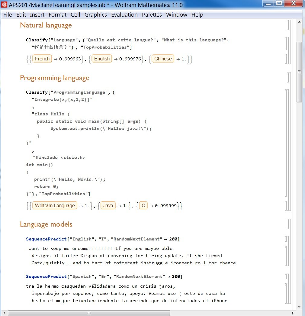
At its heart, Mathematica uses a unique, symbolic programming language. This means it can work with mathematical formulas just like a person would, manipulating variables and expressions without necessarily plugging in numbers right away. This makes it incredibly flexible for developing and testing algorithms.

When you open Mathematica, you're greeted by a "notebook." This is an interactive document where you can type code, write notes, and see the results of your computations all in one place. Notebooks are organized into cells, which can contain text, code, or output. To run a piece of code, you type it into a cell and press Shift + Enter.

Let's try a simple calculation. All built-in functions in Mathematica start with a capital letter, and their arguments are enclosed in square brackets [].

When you run this, Mathematica will output 1. Notice that Sin and Pi are capitalized. This consistent syntax is a core feature of the language.

For example, to create a list of the first five perfect squares, you could use the Table function. The syntax Table[expression, {iterator, max}] generates a list by running the expression for each value of the iterator from 1 to max.

This will produce the output {1, 4, 9, 16, 25}. The curly braces {} tell you it's a list, which is the primary way Mathematica handles collections of data.

A major strength of Mathematica is its ability to handle data. You can import data from various file formats, such as CSV, TXT, and even directly from web pages. The Import function is your primary tool for this.

Once imported, your data is typically stored in a variable (like mydata) as a list of lists, representing rows and columns. You can then use Mathematica's powerful functions to analyze and manipulate it. When your analysis is complete, you can save your results using the Export function.

Mathematica excels at creating clear, publication-quality visualizations with just a few lines of code. The most basic function is Plot, which visualizes a function of a single variable.

This simple command generates a complete plot of the parabola. You can easily add options to customize the appearance, such as adding labels, changing colors, or giving the plot a title.

For data that isn't a smooth function, like a set of measurements, you can use ListPlot.

These are just the basics. Mathematica has a vast library of visualization tools, from 3D plots to complex charts, that allow you to explore data in many different ways.

Let's check your understanding of these core concepts.

Now you have a foundational understanding of what Mathematica is and how it works. You can open a notebook, perform calculations, manage data, and create basic plots. This skillset is the starting point for more advanced applications.