Python for Data Analysis
Introduction to NumPy
The Power of Arrays
So far, we've used standard Python lists to hold collections of data. Lists are flexible, but they aren't built for fast numerical computations. When you need to perform mathematical operations on large sets of numbers, Python lists can be slow.
This is where NumPy comes in. It's a fundamental library for scientific computing in Python, and its core feature is the N-dimensional array, or ndarray.
NumPy (Numerical Python) is a library consisting of multidimensional array objects and a collection of routines for processing those arrays.
A NumPy array is a grid of values, all of the same type. Because they're stored in a more efficient, contiguous block of memory, operations on them are significantly faster than on Python lists. This efficiency is crucial in data science and machine learning, where you often work with massive datasets.
Creating NumPy Arrays
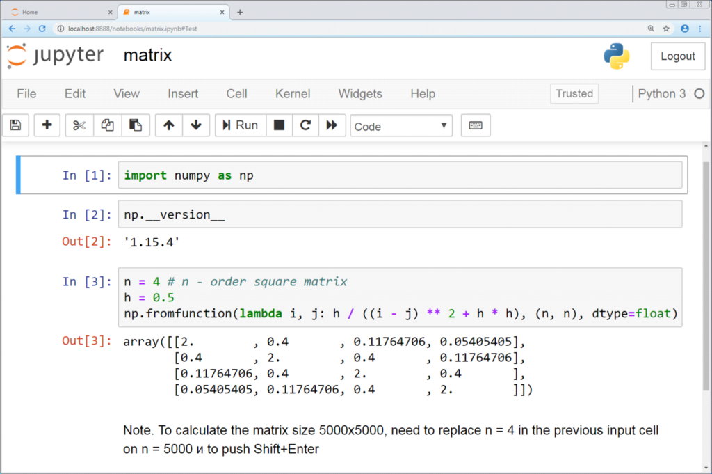
The most common way to create a NumPy array is from a Python list. To do this, you first need to import the library. By convention, it's imported with the alias np.
import numpy as np

# Create a 1D array from a list
my_list = [1, 2, 3, 4, 5]
my_array = np.array(my_list)

print(my_array)
You can also create multi-dimensional arrays by passing in a list of lists.
import numpy as np

# Create a 2D array (a matrix)
two_d_list = [[1, 2, 3], [4, 5, 6]]
matrix = np.array(two_d_list)

print(matrix)
NumPy also provides handy functions for creating arrays from scratch. For example, you can create an array filled with zeros or ones, which is useful for initializing data structures.
import numpy as np

# Create a 3x4 array of zeros
zeros_array = np.zeros((3, 4))
print(zeros_array)

# Create a 2x2 array of ones
ones_array = np.ones((2, 2))
print(ones_array)
Array Operations
One of NumPy's biggest advantages is the ability to perform element-wise operations. This means you can apply an operation to every element in an array without writing a loop. Let's say we have two arrays of the same size and we want to add them together.
import numpy as np

a = np.array([1, 2, 3])
b = np.array([10, 20, 30])

# Element-wise addition
print(a + b)  # Output: [11 22 33]

# Element-wise multiplication
print(a * b) # Output: [10 40 90]
This is much more concise and faster than looping through lists. But what happens when the arrays have different shapes? This leads to a powerful concept called broadcasting.
Broadcasting describes how NumPy treats arrays with different shapes during arithmetic operations. Subject to certain constraints, the smaller array is "broadcast" across the larger array so that they have compatible shapes.
The simplest example is operating between an array and a single number (a scalar). The scalar is stretched to match the shape of the array, and the operation is performed on every element.
import numpy as np

data = np.array([10, 20, 30, 40])

# Add 5 to every element
result = data + 5

print(result) # Output: [15 25 35 45]
This avoids the need for creating a new array like np.array([5, 5, 5, 5]). NumPy handles it automatically.
Universal Functions
NumPy provides a large library of universal functions, or "ufuncs," which are functions that operate on arrays in an element-by-element fashion. These are highly optimized and much faster than their pure Python counterparts.
For example, you can easily find the square root of every number in an array or calculate the sine of each element.
import numpy as np

numbers = np.array([0, 9, 16, 25])

# Get the square root of each element
roots = np.sqrt(numbers)
print(roots) # Output: [0. 3. 4. 5.]

# Calculate the exponential of each element
exponentials = np.exp(numbers)
print(exponentials)
Handling Missing Data
In real-world data, values are often missing. NumPy represents missing numerical data with a special value: np.nan, which stands for "Not a Number."
One important thing to know about np.nan is that it's contagious. Any arithmetic operation involving a nan value will result in nan.
import numpy as np

scores = np.array([88, 92, np.nan, 74])

# This will result in nan
print(np.mean(scores)) # Output: nan

print(np.sum(scores)) # Output: nan
This behavior can be problematic. To get around it, NumPy provides special nan-safe functions that ignore missing values when performing calculations.
import numpy as np

scores = np.array([88, 92, np.nan, 74])

# Calculate the mean, ignoring nan values
mean_score = np.nanmean(scores)
print(mean_score) # Output: 84.666...

# Calculate the sum, ignoring nan values
total_score = np.nansum(scores)
print(total_score) # Output: 254.0
Using functions like np.nanmean, np.nansum, and np.nanmin is essential for working with datasets that have missing entries.
Let's check your understanding of these core concepts.
What is the primary advantage of using a NumPy ndarray over a standard Python list for numerical computations?
What is the result of the following NumPy operation?
import numpy as np
arr = np.array([10, 20, 30, 40])
result = arr / 10
You've now seen the fundamentals of NumPy. This library is the bedrock for many other data science tools, providing a fast and efficient way to work with numerical data.