Probability is simply a way to measure how likely something is to happen. We use it every day, whether we're checking the weather forecast or deciding if we should buy a lottery ticket. It gives us a framework for thinking about uncertainty.

For many simple situations, we can calculate the exact probability of an event using a straightforward formula. An event is just a specific outcome we're interested in.

Let's use a standard six-sided die as an example. What's the probability of rolling a 3? There's only one way to roll a 3. There are six possible outcomes in total (1, 2, 3, 4, 5, or 6). So, the probability is $1/6$.

To calculate probabilities, we first need to know all the things that could happen. This complete set of all possible outcomes is called the sample space.

For our six-sided die, the sample space is {1, 2, 3, 4, 5, 6}. For a coin flip, it's {Heads, Tails}.

An event is a subset of the sample space—it's the specific outcome or group of outcomes we care about. For example, if we're interested in rolling an even number on a die, our event is the set {2, 4, 6}. There are three outcomes in this event.

The way we model probability depends on the type of data we're working with. Outcomes can be either discrete or continuous.

When we plot the probabilities for each outcome of a discrete variable, we get a probability mass function (PMF). It shows a probability value for each distinct outcome.

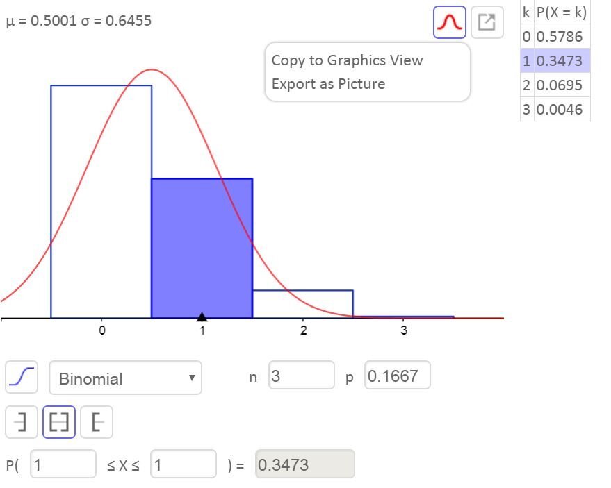
Continuous data, on the other hand, can take any value within a range. Think of someone's height, the temperature outside, or the exact time it takes to run a mile. These aren't restricted to specific, separate numbers. A person can be 1.75 meters tall, or 1.751, or 1.7512...

For continuous data, the probability of any single exact value is practically zero. What's the probability that a runner finishes a race in exactly 10.3456789... seconds? It's infinitesimal. Instead, we look at the probability of the outcome falling within a certain range, like between 10.3 and 10.4 seconds.

Understanding these basic building blocks is the first step. They allow us to create models that help us analyze risk and make more informed decisions in a world full of uncertainty. Let's test your understanding of these core ideas.