To accurately quantify carbon stocks, we can't just use raw data from different satellites. Each sensor—whether it's radar, optical, or LiDAR—captures information with its own unique quirks and distortions. Our first job is to correct these issues, creating a clean, comparable set of data layers. This process is called preprocessing, and it's about ensuring we're comparing apples to apples when we later analyse the information from Sentinel-1, Landsat, and GEDI.

Synthetic Aperture Radar (SAR) data, like that from Sentinel-1, is powerful because it can see through clouds. However, it's also highly sensitive to topography. A steep hillside facing the sensor will reflect the radar signal much more strongly than a flat plain or a slope facing away. This isn't a true reflection of the ground cover, but an artifact of the viewing angle and the landscape's shape.

To fix this, we perform radiometric terrain correction. The first step is radiometric calibration, which converts the raw digital numbers from the sensor into a standardised measure of radar backscatter. This ensures the brightness values are physically meaningful. Next, we use a Digital Elevation Model (DEM) to correct for the geometric distortions caused by terrain. This process, often called terrain flattening, adjusts the backscatter values to simulate what the sensor would have recorded over a flat surface. This removes the topographic effect, so the remaining signal variation is due to features we care about, like forest structure or soil moisture.

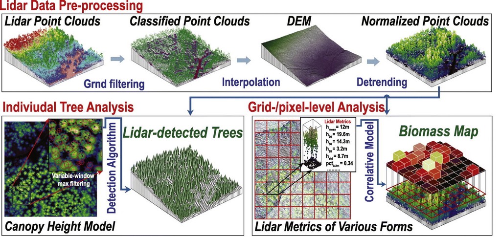
LiDAR data, which comes as a massive collection of points called a point cloud, gives us direct 3D measurements of the surface. To make sense of it, we first need to classify these points. Algorithms filter the cloud to distinguish points that hit the bare ground from those that hit vegetation, buildings, or other features.

The ground points are used to create a Digital Terrain Model (DTM), which represents the Earth's surface without any objects on it. All the points together, including vegetation, are used to generate a Digital Surface Model (DSM). The difference between these two models gives us what we're really after: the Canopy Height Model (CHM), which maps the height of the trees.

For optical imagery from satellites like Landsat-8/9 and Sentinel-2, the main hurdle is the atmosphere. Clouds, water vapour, and aerosols scatter and absorb sunlight, altering the colours and brightness values recorded by the sensor. Atmospheric correction algorithms model these effects and remove them, converting the top-of-atmosphere reflectance to a more accurate bottom-of-atmosphere, or surface, reflectance. This gives us a clearer view of the true spectral signature of the vegetation on the ground.

With each dataset individually corrected, the final step is to make them all align perfectly. This process, called co-registration, ensures that a pixel at a specific coordinate in the Landsat image corresponds to the exact same location in the Sentinel-1 SAR image and the LiDAR-derived CHM. Even small misalignments can ruin a spatial analysis.

We also need to standardise their resolution. A Landsat image might have 30-metre pixels, while our CHM could have 1-metre pixels. To combine them, we must resample all datasets to a common grid. This usually means either degrading the high-resolution data to match the coarsest layer or using more advanced methods to preserve detail. This creates a multi-temporal data stack where every pixel across every layer and every time step is perfectly aligned and ready for analysis.

Special attention is paid to the GEDI data. Its Level 2A and 2B products provide detailed information about canopy height and profile within its footprints. These footprints aren't a continuous grid but rather a series of points along the satellite's track. Integrating this data involves associating each GEDI shot with the corresponding pixels from our raster data stack (SAR, optical, and LiDAR-derived layers). This fusion of different data types is what allows us to build robust models for carbon quantification.

Now that the data is clean and aligned, we can begin the process of analysis and modelling.