We often use a single number, like the mean, to summarize a whole set of data. But that single number hides a lot of the story. Imagine two cities with the same average daily temperature. In one city, the temperature is mild all year. In the other, the summers are scorching and the winters are freezing. The average is the same, but the experience of living there is completely different.

This is where probability distributions come in. They show us the full picture: how data is spread out, what values are likely, and what values are rare. Instead of just a summary, we get the entire landscape.

To describe the spread of data, we use two key measures: variance and standard deviation. They are closely related. Variance measures the average squared difference of each data point from the mean. A larger variance means the data is more spread out.

However, because variance is in squared units (like "squared centimeters"), it can be hard to interpret. So, we take its square root to get the standard deviation. The standard deviation is in the same units as the original data, making it much more intuitive. It tells us, on average, how far each data point is from the mean.

Many things in the world, from human height to measurement errors, follow a specific pattern: the normal distribution. You might know it as the "bell curve." It's symmetrical, with most values clustering around the central peak (the mean) and tapering off equally in both directions.

A normal distribution is completely defined by just two parameters: its mean (μ) and its standard deviation (σ). The mean sets the center of the curve, and the standard deviation determines how wide or narrow it is.

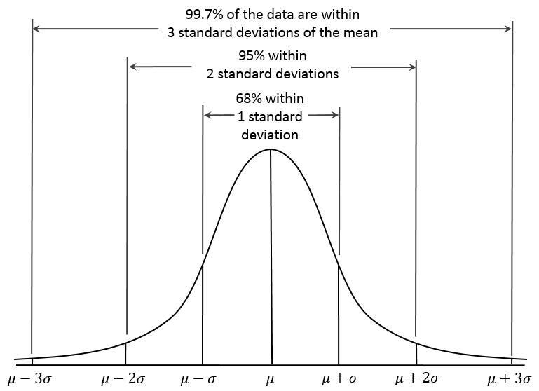
This leads to a handy guideline called the Empirical Rule (or the 68-95-99.7 rule). For any normal distribution:

• About 68% of the data falls within 1 standard deviation of the mean.
• About 95% falls within 2 standard deviations.
• About 99.7% falls within 3 standard deviations.

This rule is incredibly useful for quickly getting a feel for where most of the data lies.

To make comparing different normal distributions easier, we use the standard normal distribution. This is a special normal distribution with a mean of 0 and a standard deviation of 1. We can convert any value from a normal distribution into a "Z-score," which tells us how many standard deviations it is away from the mean.

The normal distribution is continuous; it can take on any value within a range. But what about when outcomes are countable, or discrete? For these situations, we use different distributions.

The binomial distribution is defined by two parameters: n (the number of trials) and p (the probability of success on a single trial). For example, if you flip a fair coin 10 times, you can use a binomial distribution (with n=10 and p=0.5) to find the probability of getting exactly 7 heads.

The Poisson distribution is useful for modeling events that happen independently and at a constant average rate. It's defined by a single parameter, lambda (λ), which is the average number of events in the interval. For instance, if a coffee shop serves an average of 20 customers per hour, the Poisson distribution can help calculate the probability of serving exactly 25 customers in the next hour.

Why is the normal distribution so special? Part of the answer lies in one of the most important ideas in all of statistics: the Central Limit Theorem (CLT).

The CLT states something remarkable: if you take sufficiently large random samples from any population (even a very skewed one) and calculate the mean of each sample, the distribution of those sample means will be approximately normal. This is a huge deal. It allows us to use the properties of the normal distribution to make inferences about a population, even when we don't know what the population's distribution looks like.

Finally, real-world data isn't always perfectly symmetrical. We use skewness to measure the asymmetry of a distribution. A distribution skewed to the right has a long tail on the right side, while one skewed to the left has a long tail on the left. Kurtosis measures the "tailedness" of a distribution—whether the tails are heavier or lighter than a normal distribution's. These measures help us understand how data deviates from the perfect bell curve.