Practical Machine Learning Fundamentals
Supervised Learning Fundamentals
From One Variable to Many
You're already familiar with simple linear regression, where we predict a continuous outcome using a single input variable. Think of predicting a house's price based only on its square footage. But reality is more complex. A house's price also depends on the number of bedrooms, the age of the property, and its distance from the city centre.
This is where multiple linear regression comes in. It extends the same logic to handle multiple input variables, or 'features'. Instead of finding the best-fit line in two dimensions, we're now finding the best-fit plane or hyperplane in multiple dimensions. Each feature gets its own coefficient, representing its independent contribution to the outcome.
The goal remains the same: find the specific values for the intercept () and all the coefficients ( through ) that make our model's predictions as accurate as possible.
Finding the Best Fit
How does a model 'learn' the best coefficients? It starts by making a guess, calculating how wrong its predictions are, and then adjusting its coefficients to be less wrong. This process is repeated thousands of times until the error is as low as possible.
The measure of 'wrongness' is defined by a cost function. For linear regression, the most common one is the Mean Squared Error (MSE). It calculates the average of the squared differences between the predicted values and the actual values. We square the errors so that negative and positive errors don't cancel each other out, and to penalise larger errors more heavily.
To minimise this cost, we use an optimisation algorithm called Gradient Descent. Imagine the cost function as a giant, hilly landscape where the lowest point represents the minimum possible error. Gradient Descent is like a hiker trying to find that lowest point in the fog. They take a step, check the slope (the gradient) of the ground beneath their feet, and then take their next step in the steepest downhill direction. They repeat this, taking steps of a certain size (the 'learning rate'), until they reach the bottom of a valley.
If the learning rate is too small, the hiker takes tiny steps and might take forever to reach the bottom. If it's too large, they might overshoot the valley and end up on the other side, or even bounce around erratically. Finding the right learning rate is crucial for training a model effectively.
Predicting Categories, Not Numbers
Linear regression is great for predicting continuous values like price or temperature. But what if we want to predict a category? For example, will a customer churn (yes/no), or is an email spam (spam/not spam)? These are binary classification problems.
We can't just use linear regression here. A line of best fit could produce predictions like 1.5 or -0.2, which don't make sense as 'yes' or 'no' answers. We need a model that outputs a probability, a value between 0 and 1.
Enter . Despite its name, it's a classification algorithm. It works by taking the linear equation we've already seen and passing its output through a special function called the sigmoid function.
The output of the sigmoid function is interpreted as the probability of the positive class. For instance, if we're predicting spam and the model outputs 0.8, it's 80% confident the email is spam. We can then set a threshold (typically 0.5) to make a final decision: if the probability is greater than 0.5, we classify it as spam; otherwise, we don't.
The Balancing Act
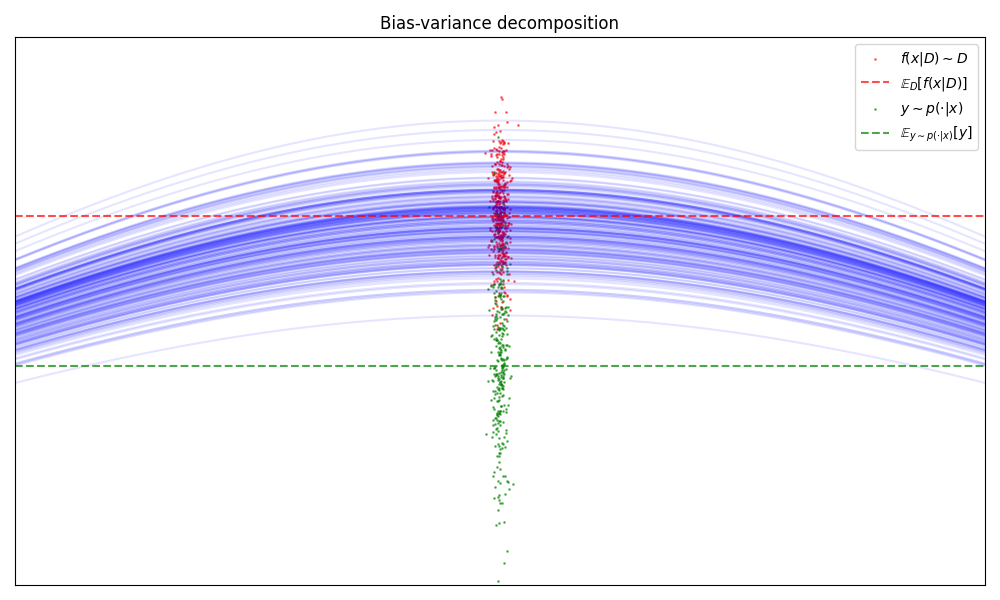
The ultimate goal isn't just to build a model that's accurate on the data it was trained on; it must also generalise well to new, unseen data. This challenge is at the heart of the .
Think of a student preparing for an exam.
- High Bias (Underfitting): The student only learns a few high-level concepts and doesn't study the details. They perform poorly on the practice questions and the final exam. Their model of the material is too simple.
- High Variance (Overfitting): The student memorises the exact answers to every single practice question. They ace the practice test, but when the final exam has slightly different questions, they fail. Their model is too complex; they've learned the noise (the specific questions) instead of the signal (the underlying concepts).
A good model, like a good student, finds the right balance. It learns the general patterns without memorising the noise in the training data.
An overfit model has learned the training data too well, including its random fluctuations or noise. An underfit model is too simplistic and fails to capture the underlying trend of the data. The challenge is to create a model that is just right.
Keeping Models in Check
One of the most effective ways to combat overfitting is through regularisation. This technique discourages model complexity by adding a penalty to the cost function. This penalty is based on the size of the model's coefficients. A complex model with large coefficients will incur a larger penalty, so the optimisation process is incentivised to keep the coefficients small.
There are two common types of regularisation:
-
Ridge Regression (L2 Regularisation): Adds a penalty equal to the sum of the squared coefficients. This forces the weights to be small, but it rarely forces them to be exactly zero. It's useful when you believe most of your features are relevant to the outcome.
-
(L1 Regularisation): Adds a penalty equal to the sum of the absolute value of the coefficients. This is a bit stricter. It can shrink some coefficients all the way to zero, effectively removing those features from the model. This makes Lasso a powerful tool for automatic feature selection.
| Technique | Penalty Term Added to Cost Function | Effect on Coefficients |
|---|---|---|
| Ridge (L2) | Shrinks coefficients towards zero. | |
| Lasso (L1) | $ \lambda \sum_{j=1}^{p} | b_j |
In both formulas, (lambda) is a hyperparameter that you tune. It controls the strength of the penalty. A larger results in smaller coefficients and a simpler, less-overfit model. By applying these techniques, we can build models that are not only accurate but also robust.
What is the primary purpose of the sigmoid function in logistic regression?
A data scientist trains a model that achieves 99% accuracy on the training data but only 65% accuracy on new, unseen test data. This is a classic example of:
These foundational techniques, from handling multiple inputs to controlling model complexity, are the building blocks for creating powerful and reliable predictive models.