Practical Machine Learning and Model Optimization
Advanced Algorithmic Intuition
The Logic of Boosting
Gradient Boosting Machines (GBMs) don't build one massive, complex model. Instead, they build a strong predictor by adding a series of simple models, usually decision trees, in a sequential fashion. Each new tree is built to correct the errors made by the previous ones. It's like a team of specialists, where each one addresses the mistakes of the one before them.
The core of this process is minimizing a loss function. For a set of predictions and actual values , we want to find the model that minimizes the total loss. A common choice for regression is the Mean Squared Error (MSE).
The secret to Gradient Boosting lies in how it corrects errors. It doesn't just look at the difference between the prediction and the actual value. Instead, it calculates the gradient of the loss function with respect to the previous prediction. These gradients are called , and they point in the direction of steepest descent for the loss. Each new tree is trained to predict these pseudo-residuals, not the original target values.
The model is built additively. If is our model after trees, we add a new tree to get the updated model :
The Art of Separation
Support Vector Machines (SVMs) approach classification differently. Their goal is to find the single best boundary, or hyperplane, that separates data points into classes. The "best" hyperplane isn't just one that separates the data, but the one that does so with the largest possible margin—the widest possible street between the closest points of each class.
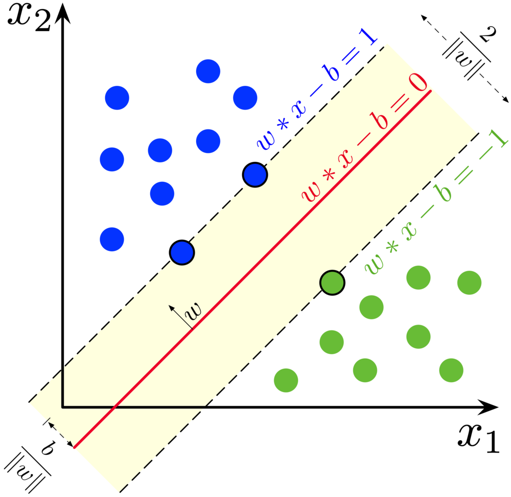
This problem of maximizing the margin is a constrained optimization problem. We want to maximize the margin subject to the constraint that all data points are classified correctly. To solve this, SVMs use a powerful mathematical tool: . This technique converts the constrained problem into an unconstrained one, making it easier to solve. This conversion process leads to a "dual" formulation of the problem, which has a fascinating property: the solution depends only on the dot products of the feature vectors of the support vectors—the points lying on the margin.
The reliance on dot products is the key that unlocks the SVM's most powerful feature.
What if the data isn't linearly separable? You can't draw a straight line to divide the classes. This is where the comes in. The idea is to project the data into a higher-dimensional space where it is linearly separable. Imagine points on a line that can't be separated by a point; if you project them onto a 2D parabola, a simple line can then separate them.
A kernel function, , computes the dot product of the vectors in this new, higher-dimensional space. We just swap the dot product in our dual formulation with a kernel function.
| Kernel | Formula | Boundary Shape |
|---|---|---|
| Polynomial | Curved or complex shapes | |
| Radial Basis Function (RBF) | $\exp(-\gamma |
Perfect separation isn't always possible or even desirable, as it can lead to overfitting. The soft margin SVM introduces a slack variable, (xi), which allows some points to be on the wrong side of the margin, or even on the wrong side of the hyperplane. A cost parameter, , controls the penalty for these misclassifications. A small allows for a wider margin at the cost of more violations, while a large prioritizes correct classification, leading to a narrower margin.
What is the primary goal of a Support Vector Machine (SVM) when used for classification?
In a Gradient Boosting Machine (GBM), what are the subsequent simple models (like decision trees) trained to predict?
Understanding these mechanics—how GBMs chase gradients and how SVMs find optimal boundaries in other dimensions—is the difference between simply using a model and truly engineering a solution.