Pandas Data Wrangling

From Raw to Ready

Data rarely arrives in a tidy format. More often, it's a messy collection of files that need to be cleaned, combined, and restructured before any real analysis can begin. This process is called data wrangling, and it's where most of the work in data science happens. At the heart of efficient data wrangling in Python are two libraries: NumPy and Pandas.

NumPy introduces the concept of vectorization, which is a fancy way of saying you can perform operations on entire arrays of data at once, rather than looping through each element individually. This is dramatically faster because the operations are executed in pre-compiled C code. Pandas is built on top of NumPy and brings this performance to a more flexible data structure designed for real-world data.

import numpy as np

# Without vectorization (slow)
a = [1, 2, 3, 4]
b = [5, 6, 7, 8]
result = []
for i in range(len(a)):
    result.append(a[i] + b[i])

# With NumPy vectorization (fast)
a_np = np.array([1, 2, 3, 4])
b_np = np.array([5, 6, 7, 8])
result_np = a_np + b_np # Clean and fast

print(result_np)
# Output: [ 6  8 10 12]

The DataFrame

The core of Pandas is the , a two-dimensional labeled data structure that looks a lot like a spreadsheet or a SQL table. It has rows and columns, and both can have labels. The row labels are called the index, and the column labels are simply called columns. This structure allows for intuitive and powerful ways to select, filter, and manipulate data.

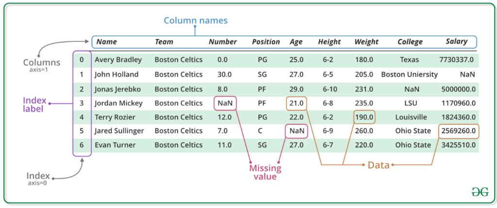
You can select data from a DataFrame using its labels or its integer position. For label-based selection, you use the .loc indexer. For position-based selection, you use .iloc.

import pandas as pd

data = {'Name': ['Alice', 'Bob', 'Charlie', 'David'],
        'Age': [25, 30, 35, 40],
        'City': ['New York', 'Los Angeles', 'Chicago', 'Houston']}
df = pd.DataFrame(data, index=['a', 'b', 'c', 'd'])

# Label-based selection with .loc
print(df.loc['b'])

# Position-based selection with .iloc
print(df.iloc[2])

# Selecting a specific cell (row 'c', column 'City')
print(df.loc['c', 'City']) # Outputs: Chicago

# Slicing rows and columns
print(df.loc['b':'d', ['Name', 'City']])

A common and powerful technique is boolean indexing, which lets you filter data based on conditions. For example, df[df['Age'] > 30] would select only the rows for Charlie and David.

For more complex datasets, Pandas supports hierarchical indexing, or multi-indexing. This lets you have multiple index levels on an axis, providing a way to work with higher-dimensional data in a 2D format.

Combining Datasets

Real-world projects often require combining data from multiple sources. Pandas provides high-performance, in-memory join and merge operations that mirror the logic of SQL. The main function for this is pd.merge().

Join Type	Description
`inner`	Returns only the rows that have matching keys in both DataFrames.
`outer`	Returns all rows from both DataFrames, filling in `NaN` for missing matches.
`left`	Returns all rows from the left DataFrame, and matched rows from the right.
`right`	Returns all rows from the right DataFrame, and matched rows from the left.

# DataFrames for employees and their departments
df_employees = pd.DataFrame({
    'employee_id': ['E1', 'E2', 'E3', 'E4'],
    'name': ['Alice', 'Bob', 'Charlie', 'David'],
    'dept_id': ['D1', 'D2', 'D1', 'D3']
})

df_depts = pd.DataFrame({
    'dept_id': ['D1', 'D2', 'D4'],
    'dept_name': ['Sales', 'Engineering', 'Marketing']
})

# Perform an inner join
inner_join = pd.merge(df_employees, df_depts, on='dept_id', how='inner')
print(inner_join)
# Note: David (D3) and Marketing (D4) are excluded.

# Perform a left join
left_join = pd.merge(df_employees, df_depts, on='dept_id', how='left')
print(left_join)
# Note: David is included, but his dept_name is NaN.

GroupBy and Transform

One of the most powerful features of Pandas is the ability to perform GroupBy operations. This follows a "split-apply-combine" pattern: you split the data into groups based on some criteria, apply a function to each group independently, and then combine the results into a new data structure. It's essential for calculating aggregate statistics.

data = {'Team': ['A', 'B', 'A', 'B', 'A'],
        'Player': ['P1', 'P2', 'P3', 'P4', 'P5'],
        'Points': [10, 12, 8, 15, 12]}
df = pd.DataFrame(data)

# Group by team and calculate the sum of points for each
team_points = df.groupby('Team')['Points'].sum()
print(team_points)
# Output:
# Team
# A    30
# B    27
# Name: Points, dtype: int64

Sometimes, you don't want to collapse the DataFrame with an aggregation. You might want to perform a calculation on a group and then broadcast that result back to the original shape of the DataFrame. This is what the transform method is for.

For example, you could use transform to center data by subtracting the group-wise mean from each value, or to calculate the percentage of a total that each row represents.

# Calculate the total points for each team
# and show it next to each player
df['Team_Total_Points'] = df.groupby('Team')['Points'].transform('sum')

print(df)
#   Team Player  Points  Team_Total_Points
# 0    A     P1      10                 30
# 1    B     P2      12                 27
# 2    A     P3       8                 30
# 3    B     P4      15                 27
# 4    A     P5      12                 30

Mastering these techniques—indexing, merging, and grouping—forms the foundation of effective data wrangling. They allow you to take disparate, messy datasets and shape them into clean, structured inputs ready for modeling and visualization.

Quiz Questions 1/6

What is the primary advantage of using vectorization in NumPy?

Quiz Questions 2/6

In Pandas, what is the core data structure that represents a two-dimensional, labeled table with columns and a row index?

Practical Data Science Mastery