Practical Artificial Intelligence Applications
Neural Network Design
Deeper or Wider?
When designing a neural network, one of the first decisions is its shape. Should you build a tall, narrow skyscraper or a wide, single-story warehouse? This is the depth versus width trade-off.
A deeper network (more layers) can learn hierarchical features. The first layer might learn edges, the next shapes, and a later one might recognize complex objects like faces. This abstraction is powerful but comes at a cost. Deep networks are notoriously difficult to train.
A wider network (more neurons per layer) can theoretically approximate any function, but it might not learn the elegant, hierarchical representations that lead to better generalization. It can also be computationally expensive, as the number of parameters explodes with width.
The choice isn't either/or. The best architectures often balance depth and width, creating a structure that is both expressive and trainable.
Predicting Performance
It would be ideal to know if a network architecture is promising before spending hours on training. The (NLC) offers a way to do just that. It's a metric that quantifies the expressive power of a network based on its structure.
The NLC measures a network’s capacity to model complex, non-linear relationships. A higher NLC suggests the network can fit more intricate patterns in the data. However, too high an NLC can be a red flag for overfitting, where the model learns the training data's noise instead of the underlying signal.
By calculating the NLC, you can gauge whether your proposed architecture has enough capacity to model the problem without being excessively complex. A model with a low NLC might underfit, failing to capture the data's patterns, while one with a very high NLC might overfit dramatically.
The Problem with Deep Networks
As we stack more and more layers, a serious problem emerges: the vanishing gradient. During backpropagation, the error signal is multiplied by the gradient of each layer as it travels backward through the network. In a deep network, this repeated multiplication can cause the gradient to shrink exponentially, becoming so small that the early layers learn extremely slowly, or not at all.
This effectively freezes the weights in the initial layers, preventing the network from learning those crucial low-level features. The solution is surprisingly simple: give the gradient a shortcut.
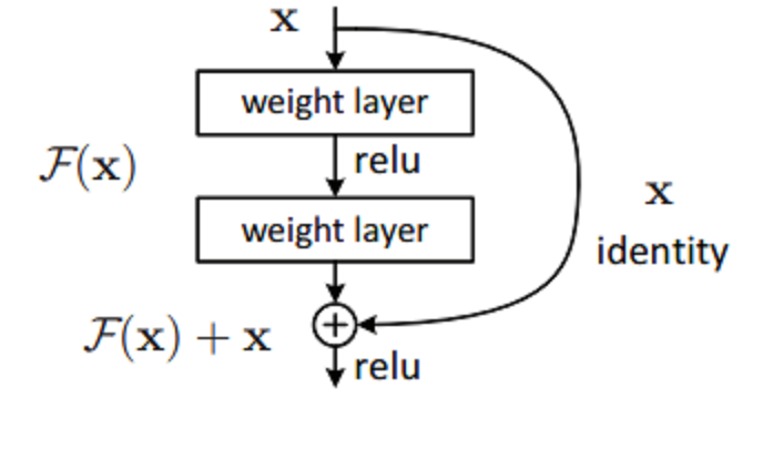
This is the idea behind (also called skip connections). Instead of forcing the signal to pass sequentially through every layer, we add the input of a block, , directly to its output, . The new output is .
This simple addition creates an uninterrupted highway for the gradient to flow through the network. The network is no longer forced to learn a complete transformation from scratch; instead, it only needs to learn the residual, or the difference between the desired output and the input. This innovation made it possible to train networks with hundreds or even thousands of layers.
Smart Starting Points
A good architecture is only half the battle. How you initialize the network's weights is just as critical. A poor initialization can stall learning before it even begins. The goal of is to set the initial weights so that the signal—both forward during inference and backward during training—flows properly without exploding or vanishing.
| Initializer | Key Idea | Best For | Formula (Variance ) |
|---|---|---|---|
| Xavier / Glorot | Keeps activation variance consistent across layers. | Symmetric activations like tanh, sigmoid. | |
| He | Accounts for ReLU cutting half the activations. | ReLU and its variants (Leaky ReLU, GeLU). |
Xavier (or Glorot) initialization was designed to keep the variance of the activations and gradients constant across layers. It works well for activation functions that are symmetric around zero, like tanh. However, it struggles with the non-symmetry of ReLU.
He initialization solves this. Since ReLU sets all negative inputs to zero, it effectively halves the variance of its outputs. He initialization accounts for this by doubling the output variance, drawing weights from a distribution with variance , where is the number of input neurons to the layer. This simple change helps keep the signal flowing in deep ReLU-based networks.
Choosing an Activation Function
The Rectified Linear Unit (ReLU) is the default choice for many networks due to its simplicity and effectiveness. But modern architectures often benefit from more advanced activation functions.
| Function | Formula | Pro | Con |
|---|---|---|---|
| ReLU | Computationally cheap, avoids vanishing gradients. | Can "die" if neuron output is always negative. Not smooth. | |
| GeLU | Smooth, performs well in Transformers. | More computationally expensive than ReLU. | |
| Swish | Often performs slightly better than ReLU. Self-gated. | Also more expensive than ReLU. |
The Gaussian Error Linear Unit (GeLU) is a smooth approximation of ReLU. Instead of a hard gate at zero, it weights inputs based on their value, creating a smoother curve. This property is particularly useful in Transformer models like BERT and GPT.
Swish is another smooth alternative that often outperforms ReLU. It's a self-gated function, meaning the function itself learns whether to activate a neuron or not. The parameter can even be made learnable. Both GeLU and Swish offer small but consistent improvements over ReLU in very deep models, at the cost of slightly more computation.
What is the primary advantage of building a "deep" neural network (many layers) compared to a "wide" one (many neurons per layer)?
A network with a very high Nonlinearity Coefficient (NLC) is at risk of __________, while a network with a very low NLC might __________.
Designing a neural network is an art informed by science. By understanding the trade-offs between depth and width, using tools like NLC, and making smart choices about residual connections, initialization, and activation functions, you can build powerful models that train efficiently and generalize well.