We often think of PCA as a tool for reducing dimensions or visualizing data. But it has another powerful identity: it's an effective signal filter. Any dataset with meaningful structure also contains random fluctuations, or noise. PCA provides a systematic way to separate the two.

The core idea is to partition your data into two distinct spaces. The first is the signal subspace, which contains the dominant patterns and correlations—the essential information. The second is the noise subspace, which captures the random, high-frequency variations that often obscure the underlying structure. By projecting your data onto the signal subspace, you effectively filter out the noise.

How does PCA actually perform this filtering? The mechanism is orthogonal projection onto a lower-dimensional basis. As you know, the principal components form a new, orthogonal basis for your data, ordered by the amount of variance they explain. The first few components capture the broad strokes—the signal. The last few components typically represent the fine-grained, stochastic noise because random noise tends to be spread out in all directions, contributing a small amount of variance to many dimensions.

When you reduce the rank of your dataset—that is, you decide to keep only the top $k$ principal components—you are making an explicit choice. You are projecting your original data from its high-dimensional space onto the lower-dimensional signal subspace defined by those $k$ components. The information contained in the discarded components is treated as noise and left behind.

This visual demonstrates how projecting the data effectively squashes the variance along the third principal component. We've defined this axis as our noise dimension and removed its influence, leaving a cleaner representation of the signal.

The eigenvalues of the covariance matrix become our guide in this process. Since each eigenvalue corresponds to the variance captured by its respective principal component, you can interpret them as indicators of signal strength.

Plotting the eigenvalues in descending order, known as a scree plot, often reveals an "elbow" point. The components before the elbow are typically considered the signal, while those after represent the noise floor of the data. This provides a principled way to decide where to make the cut—how many components to keep to preserve the signal while discarding the maximum amount of noise.

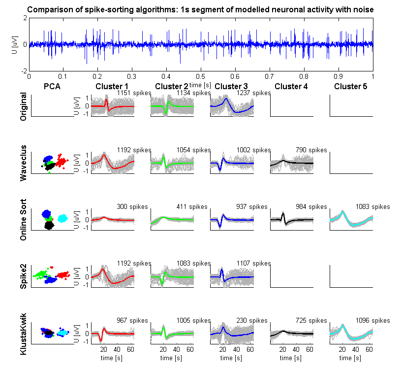
This image shows a real-world example from neuroscience. Raw brain activity is noisy. By applying PCA, researchers can cluster the data points. Each cluster represents the unique electrical "signature" or signal from a single neuron, effectively filtered from the noisy recordings of many neurons firing at once.

By shifting our view of PCA from a simple visualization tool to a sophisticated filter, we can use it to preprocess data for machine learning models. A model trained on signal-rich, noise-reduced data will often perform better, generalize more effectively, and train faster. It’s a powerful first step in any serious data analysis pipeline.