Neural Networks and the Mechanics of Backpropagation
Network Dynamics and Flow
From Neuron to Network
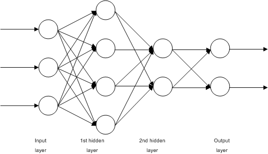
You already know that neural networks are composed of layers, which are themselves collections of individual neurons. But how does information actually move through this structure? The process is a highly organized, one-way street called the forward pass or forward propagation.
Think of it like an assembly line. Raw data enters at one end, and at each station (layer), it gets transformed. The output of one station becomes the input for the next, until a final, processed output emerges at the end. This entire journey from input to output is the forward pass. It's the network's way of making a prediction based on what it currently knows.
The Math of the Message
To process data efficiently, we don't calculate one neuron at a time. Instead, we use the language of linear algebra: vectors and matrices. The input data is a vector, and all the connection weights for a layer are organized into a single matrix. This allows us to compute the transformations for an entire layer in one go.
Each layer performs two main operations. First, it applies a linear transformation to its input. We take the input vector (), multiply it by the layer's weight matrix (), and add a bias vector (). This gives us an intermediate result, often called the pre-activation state or "logits," which we'll label .
This equation is the workhorse of the network. It takes the input data, which exists as a point in a high-dimensional space, and rotates, stretches, and shifts it to a new position. The weight matrix handles the rotation and stretching, while the bias vector handles the shift.
The second operation introduces the crucial non-linearity. The pre-activation vector is passed through an activation function (represented by , the Greek letter sigma) to produce the layer's final output, the post-activation state, . This step is what allows the network to learn complex patterns that a purely linear model could not.
Chaining Layers Together
The real power of deep learning comes from stacking these layers. The post-activation output vector from one layer becomes the input vector for the very next layer. This creates a chain of transformations, where the data is progressively refined as it flows through the network.
For this chain to work, the dimensions of the vectors and matrices must align perfectly. The number of columns in a layer's weight matrix must equal the number of neurons in the previous layer (the size of its input vector). The number of rows must equal the number of neurons in the current layer (the size of its output vector).
If Layer 1 has 784 neurons and Layer 2 has 128 neurons, the weight matrix connecting them, , must have the dimensions 128x784.
| Layer | Number of Neurons | Input Vector Size | Weight Matrix Dimensions | Output Vector Size |
|---|---|---|---|---|
| Input (Layer 0) | 784 | N/A | N/A | 784 |
| Hidden 1 | 128 | 784 | 128 x 784 | 128 |
| Hidden 2 | 64 | 128 | 64 x 128 | 64 |
| Output (Layer 3) | 10 | 64 | 10 x 64 | 10 |
This sequence of nested operations means we can think of the entire network as one large, composite function. If , , and represent the operations of each layer, the network's final output is . Understanding the network in this way is the key that unlocks how we can train it using calculus, which we'll explore next.