Monte Carlo Simulations Explained
Introduction to Probability
Understanding Randomness
Life is full of uncertainty. Will it rain tomorrow? Will your favorite team win the championship? Probability is the branch of math that helps us measure and reason about this uncertainty. It gives us a framework for understanding random events.
A random event has multiple possible outcomes. Flipping a coin can result in heads or tails. Rolling a die can yield any number from one to six. A probability distribution is a way of mapping every possible outcome of a random event to its likelihood of happening.
Think of a probability distribution as a complete guide to the chances of every possible result.
For a fair six-sided die, each outcome (1, 2, 3, 4, 5, or 6) has an equal chance of occurring. The probability for each is $1/6$. We can show this in a simple table.
| Outcome | Probability |
|---|---|
| 1 | 1/6 |
| 2 | 1/6 |
| 3 | 1/6 |
| 4 | 1/6 |
| 5 | 1/6 |
| 6 | 1/6 |
This is a simple probability distribution. The probabilities of all possible outcomes must always add up to 1, because it's certain that one of the outcomes will happen.
Not all distributions are uniform like the die roll. Imagine a loaded die that's twice as likely to land on 6. The probabilities would shift, but they would still sum to 1. This shows how distributions can describe all sorts of random phenomena, from fair games to biased ones.
Expected Value and Variance
Once we have a probability distribution, we can start to describe its properties. Two of the most important are the expected value and the variance.
The expected value is the long-run average outcome we would anticipate if we repeated the random event many, many times. It's a weighted average, where each outcome is weighted by its probability. You can think of it as the 'center' of the distribution.
average
noun
A number expressing the central or typical value in a set of data, in particular the mode, median, or (most commonly) the mean.
The formula for the expected value, denoted , is the sum of each outcome multiplied by its probability.
Let's calculate it for our fair die. Each outcome is a number from 1 to 6, and each probability is .
Even though you can't roll a 3.5, if you rolled the die thousands of times and averaged the results, your average would be very close to 3.5.
While expected value tells us about the center of a distribution, variance tells us about its spread. Are the outcomes tightly clustered around the expected value, or are they widely scattered?
A low variance means the outcomes are predictable and consistent. A high variance means they are unpredictable and spread out.
Variance, denoted , is calculated by taking the average of the squared differences from the Expected Value. A small variance means most outcomes are close to the average; a large variance means they are far from it.
Consider two different games. In Game A, you win $10 every time. The expected value is $10 and the variance is 0 because the outcome never changes. In Game B, you have a 50% chance of winning $0 and a 50% chance of winning $20. The expected value is still $10, but the variance is much higher because the outcomes are spread far apart. Variance helps us understand the risk or volatility of a random process.
The Law of Large Numbers
The Law of Large Numbers is a simple but powerful idea that connects theoretical probability with real-world results. It states that as you repeat an experiment more and more times, the average of the results will get closer and closer to the expected value.
Imagine flipping a coin. The expected value of a single flip (if we say heads=1, tails=0) is 0.5. If you flip it 10 times, you might get 7 heads (an average of 0.7). This isn't very close to 0.5. But if you flip it 10,000 times, the number of heads will be very close to 5,000, and the average will be extremely close to 0.5.
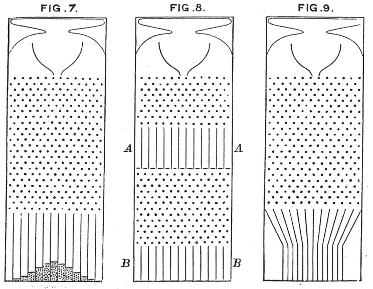
This principle is the bedrock of statistics and simulations. It's the reason casinos can be certain of their profits over the long run, even though individual bets are unpredictable. It’s also why we can trust a large political poll to reflect the opinion of an entire country. With enough trials, the randomness starts to form a predictable pattern.
The Central Limit Theorem is one of the most important concepts in statistics.
The Law of Large Numbers guarantees that with a large enough sample size, the sample average will converge to the true average of the population. This reliability is what makes it possible to model complex systems by running many simulations and averaging the results.
Ready to check your understanding? Let's try a few questions.
What must the probabilities of all possible outcomes in a probability distribution always sum to?
A game gives you a 25% chance of winning 0. What is the expected value of playing this game?
These concepts of probability, expected value, and variance are the basic building blocks for understanding more advanced topics. They give us the tools to analyze and predict the behavior of random systems.