Microsoft Excel Mastery for Data Efficiency
Advanced Data Organization
From Ranges to Robust Tables
Working with data in loose cell ranges is like building a house on a shaky foundation. It might hold up for a while, but as your dataset grows, things start to break. Formulas don't update automatically when you add new rows, formatting becomes inconsistent, and sorting can accidentally jumble your data if you don't select the entire range perfectly.
The professional solution is to convert your data range into an official Excel Table. This simple step transforms a static grid of cells into a dynamic, structured object. To do this, just click anywhere inside your data range and press Ctrl+T (or Cmd+T on a Mac). Excel will automatically detect your data and headers.
Excel Tables automatically expand to include new rows or columns, so your formulas, charts, and PivotTables always reference the most up-to-date information.

Once you have a Table, you'll notice a new “Table Design” tab appears in the ribbon. This gives you tools for naming your table, changing styles, and adding features like a Total Row. Tables also use “structured references,” which are easier to read than standard cell addresses. Instead of =SUM(C2:C100), you might write =SUM(Sales[Amount]). This makes formulas more intuitive and less prone to errors.
Sophisticated Sorting
You're likely familiar with sorting a single column from A to Z. But real-world data often requires more nuance. Multi-level sorting allows you to apply a hierarchy to your organization. For example, you might want to see sales data organized first by region, then by salesperson, and finally by date.
To perform a multi-level sort:
- Click inside your Excel Table.
- Go to the Data tab and click 'Sort'.
- In the dialog box, set your first sorting level (e.g., 'Sort by' Region, 'Order' A to Z).
- Click 'Add Level' to add your second criterion (e.g., 'Then by' Salesperson, 'Order' A to Z).
- Continue adding levels as needed.
Sometimes, alphabetical or numerical order isn't what you need. Imagine you have a column with product sizes (Small, Medium, Large) or project statuses (Low, Medium, High). Sorting alphabetically would produce an illogical order. This is where custom lists come in. You can define your own sorting sequence that Excel will remember and apply.
| Unsorted | A-Z Sort | Custom List Sort |
|---|---|---|
| Medium | High | Low |
| High | Low | Medium |
| Low | Medium | High |
| Medium | Medium | Medium |
To create a custom list, go to File > Options > Advanced. Scroll down to the 'General' section and click 'Edit Custom Lists...'. Here, you can type your list items in the desired order (e.g., Low, Medium, High). Once saved, this list will appear as an option in the 'Order' dropdown of the main Sort dialog box.
Filtering with Precision
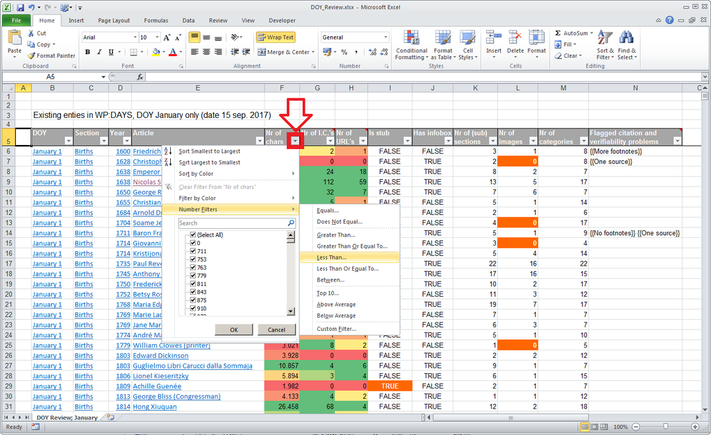
Filtering is essential for focusing on specific subsets of your data. While the filter dropdowns in a Table's header row are useful, they can be cumbersome when you need to frequently change criteria. For a more interactive experience, use slicers.
Slicers are visual filters. They are essentially large buttons that let you quickly and easily filter your Table data. To add one, click inside your Table, go to the 'Table Design' tab, and click 'Insert Slicer'. Choose the column(s) you want to filter by, and Excel will create floating slicer panels for each.
With slicers, you can see at a glance what filters are currently active. Clicking a button on a slicer instantly filters the table. You can select multiple items by holding down the Ctrl key. Slicers make your spreadsheets feel more like interactive dashboards, which is great for analysis and presentation.
Keeping Data Clean
Your analysis is only as good as your data. Inaccurate, inconsistent, or redundant data can lead to flawed conclusions. One of the most common data cleaning tasks is removing duplicate entries.
Imagine you have a customer list where some people have signed up more than once. To fix this, Excel provides a simple tool. Click anywhere in your Table, go to the 'Data' tab, and click 'Remove Duplicates'. A dialog box will appear, letting you choose which columns to check for duplicate values. If a row has identical values across all selected columns, it will be removed.
Data cleaning is the cornerstone of effective data analysis, and Microsoft Excel is a powerful tool for the job.
Beyond duplicates, keep an eye out for other inconsistencies. Common issues include extra spaces before or after text, which can be fixed with the =TRIM() function, or inconsistent naming (e.g., 'USA' vs 'United States'), which can be standardized using Find and Replace.
What is a primary advantage of converting a loose cell range into an official Excel Table?
You have an Excel Table named 'Sales' with a column titled 'Amount'. Which formula correctly uses a structured reference to sum all the values in that column?
By moving from simple ranges to structured Tables and using advanced tools for sorting, filtering, and cleaning, you create a reliable foundation for any analysis you perform.