Merging Excel Data
Excel Tables
Beyond the Grid
Most people use Excel as a simple grid of cells. You type in some data, maybe add a formula here and there, and that's it. But to really manage information, you need to use one of Excel's most fundamental features: a Table.
An Excel Table isn't just a block of cells with formatting. It's a structured container that tells Excel, "Hey, all this data belongs together." Think of a normal range of data as a pile of business cards on your desk. You can see the information, but finding a specific card or sorting them by last name is a manual chore.
Converting that range into an Excel Table is like putting all those cards into a digital contacts app. Each piece of information (name, company, phone number) is now in a distinct field. This structure makes managing your data much, much easier.
Tables make your data dynamic. As you add new rows, your formatting, formulas, and filters automatically expand to include them. This saves time and prevents errors.
Creating Your First Table
Let’s start with a plain range of data, like this list of monthly sales:
| Month | Salesperson | Region | Sales |
|---|---|---|---|
| January | Chen | North | $5,200 |
| February | Garcia | South | $4,800 |
| January | Smith | West | $6,100 |
| March | Chen | North | $5,500 |
| February | Smith | West | $5,900 |
To turn this into a powerful Excel Table, the process is simple:
- Click any single cell inside your data. For our example, click on 'Garcia' or '$6,100'.
- Go to the Insert tab on Excel's ribbon and click the Table button.
- A small window will pop up, confirming the data range. It will also have a checkbox that says My table has headers. Since our data has headers ('Month', 'Salesperson', etc.), make sure this is checked and click OK.
The keyboard shortcut is even faster. Just click inside your data and press Ctrl+T (or Cmd+T on a Mac).
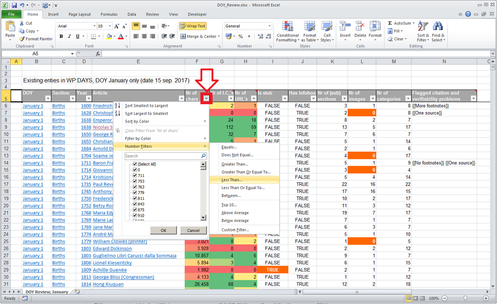
Instantly, your data will look different. It will have colored rows and, most importantly, filter buttons (small dropdown arrows) next to each header.
Basic Data Operations
Those little dropdown arrows are your new best friends. They unlock the ability to quickly organize and explore your data without complex formulas.
Sorting rearranges all your data based on the contents of one column.
Let's say you want to see the sales from largest to smallest. Click the arrow next to the 'Sales' header. You’ll see options like 'Sort Smallest to Largest' and 'Sort Largest to Smallest'. If you click the latter, the entire table rearranges to put the highest sale at the top. Notice how all the data in each row moves together—March's sale from Chen stays with March and Chen.
Filtering temporarily hides rows that don't meet your criteria.
Now, imagine you only want to see sales from the 'North' region. Click the arrow in the 'Region' header. In the menu that appears, uncheck 'Select All' and then check only the box for 'North'.
When you click OK, the rows for the South and West regions disappear. They aren't deleted, just hidden. The row numbers on the left will turn blue, indicating a filter is active. To see all your data again, just go back to the same menu and click 'Clear Filter From "Region"'.
Mastering these two simple operations—sorting and filtering—is the first step toward using spreadsheets for powerful data analysis. They allow you to quickly answer questions and spot patterns in your information.
What is the primary advantage of converting a range of data into an Excel Table?
To turn a data range into an Excel Table, you should select a cell within the data, then navigate to the 'Insert' tab and click the 'Table' button.
These foundational skills are what you'll build on as you start working with more complex datasets.