Algebra is more than just solving for $x$. It's the study of relationships and structure. You already know how to work with linear equations, where variables have a straightforward, one-to-one relationship. But the real world is rarely that simple. We'll now explore how variables interact in more complex systems, starting with polynomials.

A polynomial is just an expression with multiple terms, like $x^3 - 4x^2 + 2x - 8$. Finding the roots of such an expression—the values of $x$ that make it equal to zero—reveals its fundamental behavior. While you've likely factored simple quadratics, more complex polynomials require different strategies. One powerful method is factoring by grouping.

This technique works because it uncovers a shared structure within the polynomial. Not all polynomials can be factored this way, but it's a great example of looking for patterns beyond simple trinomials. Other patterns, like the sum and difference of cubes, provide shortcuts for factoring higher-order polynomials.

Another way to think about algebraic relationships is through functions. A function is like a machine that takes an input and produces a specific output. We use functional notation, like $f(x)$, to describe this process. The letter $f$ is the name of the function, and $x$ is the input variable.

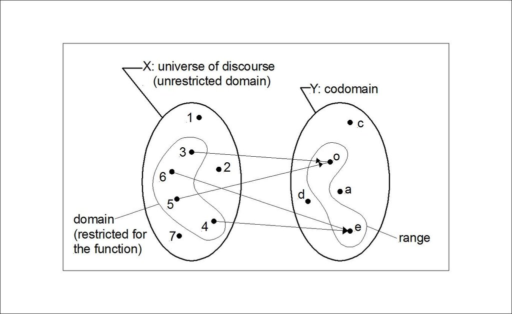
For example, the function $f(x) = x^2 + 3$ takes any number $x$, squares it, and adds 3. If you input $2$, the output is $f(2) = 2^2 + 3 = 7$. If you input $-4$, the output is $f(-4) = (-4)^2 + 3 = 19$. This notation is a powerful way to represent cause and effect. It's the language we use to model everything from the trajectory of a baseball to the growth of a bank account.

A key application of functions is modeling physical motion. When you throw a ball, its height over time can be described by a quadratic function, often of the form $h(t) = -gt^2 + v_0t + h_0$, where $t$ is time, $g$ is the acceleration due to gravity, $v_0$ is the initial upward velocity, and $h_0$ is the initial height. Here, the function $h(t)$ doesn't just give us a number; it describes the complete path of the ball. The negative sign on the $t^2$ term is what creates the characteristic arc, or parabola, of the flight path.

What happens when we create functions by dividing one polynomial by another? We get a rational expression. These are essentially fractions that contain variables, and they introduce a new, critical idea: constraints.

These constraints are not just mathematical oddities; they represent real-world limitations. Imagine a function describing the time it takes to travel a certain distance based on your speed, $t(s) = \frac{d}{s}$. The speed, $s$, cannot be zero. Or consider a function for the concentration of a chemical in a mixture. There might be values that are physically impossible to achieve, which would manifest as constraints in the function.

This graph shows the behavior of $f(x) = \frac{1}{x-2}$. The function shoots off to infinity and negative infinity near the vertical asymptote at $x=2$, a place the function can never touch. Understanding these constraints is a core part of algebraic reasoning. It's about seeing the boundaries and rules that govern the system you're modeling.

Let's test your understanding of these concepts.

By mastering these techniques, you move from simply calculating answers to analyzing the underlying structure of a problem. This abstract reasoning is the true power of algebra.