Mathematical Foundations of Monte Carlo Methods
Random Variable Mechanics
The Engine of Randomness
To simulate random events, we need more than just a coin flip. We need a precise way to describe and measure randomness. The two most important measures are the expected value and the variance of a random variable.
The expected value, or mean, is the long-run average value of a random variable. It's the center of the distribution.
For a discrete random variable that can take on values with probabilities , the expected value is the sum of each value multiplied by its probability.
For a continuous random variable, we can't just sum up the probabilities of individual points because the probability of any single exact value is zero. Instead, we use an integral. We integrate the variable's value, , multiplied by its probability density function, , across all possible values.
Variance measures the spread of a distribution. A low variance means the values are clustered tightly around the mean, while a high variance means they are spread out. It's formally defined as the expected value of the squared difference between the variable and its mean, .
Just like with expectation, this leads to two formulas. For discrete variables, we use a sum:
And for continuous variables, we use an integral:
Describing Randomness
Expected value and variance summarize a distribution, but they don't tell the whole story. To fully describe a random variable, we use probability functions.
For a continuous random variable, this is the Probability Density Function (PDF), denoted . The PDF doesn't give you the probability of a specific value. Instead, the area under the curve between two points gives the probability that the variable will fall within that range.
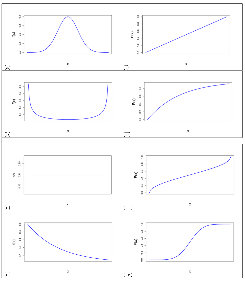
A related concept is the Cumulative Distribution Function (CDF), denoted . The CDF gives the total probability that the random variable will take on a value less than or equal to . It's the accumulated probability up to that point.
For any continuous variable, the CDF is simply the integral of the PDF from negative infinity up to .
The CDF always ranges from 0 to 1. It starts at 0 for very small values of and climbs to 1 as increases, capturing all possible outcomes.
Shaping Randomness
Computers are great at generating random numbers, but they usually produce them from a uniform distribution, where every number between 0 and 1 is equally likely. What if we need numbers that follow a normal (bell curve) distribution or some other shape?
This is where we need to transform variables. The most fundamental technique for this is the Inverse Transform Method. It's a clever way to turn uniform random numbers into random numbers from any other distribution, as long as we know its CDF.
The method works by mapping a uniform random number through the inverse of the target distribution's CDF.
Here’s the process:
- Generate a random number, , from a Uniform(0, 1) distribution.
- Find the CDF, , of the distribution you want to generate numbers from (e.g., Normal, Exponential).
- Calculate the inverse of that CDF, which we write as .
- Apply this inverse function to your random number . The result, , will be a random number that follows your target distribution.
This method is the mathematical heart of generating the random inputs needed for Monte Carlo simulations. By starting with a simple, universally available random source (the uniform distribution), we can create samples that mimic almost any random process we want to study.
| Distribution | Type | PDF / PMF | Expected Value (μ) | Variance (σ²) |
|---|---|---|---|---|
| Uniform(a, b) | Continuous | |||
| Normal(μ, σ²) | Continuous | |||
| Bernoulli(p) | Discrete | for |
Now, let's test your understanding of these core mechanics.
What does the expected value of a random variable represent?
A low variance for a random variable indicates that its values are spread out widely from the mean.
With these mathematical tools, we can precisely define, measure, and generate the randomness that powers stochastic simulations.