In machine learning, we often represent data as lists of numbers. For example, a house could be described by its square footage, number of bedrooms, and price. We can bundle these numbers into a single object called a vector. A vector isn't just a list; it's a point in a multi-dimensional space. Our house vector [2100, 3, 500000] is a single point in a 3D space where the axes are square footage, bedrooms, and price.

Vectors can be manipulated. We can add two vectors together or multiply one by a number (a scalar). Adding vectors is like adding their corresponding components. If you have two vectors representing two separate grocery trips, adding them gives you a total grocery vector. Multiplying a vector by a scalar stretches or shrinks it. If you double your grocery trip, you multiply your vector by 2.

The collection of all possible vectors of a certain type (e.g., all 3D vectors) forms a vector space. Think of it as the universe where these vectors live and interact according to the rules of vector addition and scalar multiplication.

If vectors are lists of numbers, matrices are grids of numbers, arranged in rows and columns. A dataset can be represented as a matrix, where each row is a data point (like our house vector) and each column is a feature (square footage, bedrooms, etc.).

Like vectors, matrices can be added and multiplied by scalars. These operations happen element-by-element, just as you'd expect. Matrix multiplication, however, is different and more powerful. It's not an element-by-element multiplication. Instead, it involves a row-by-column dot product operation. The element in the first row and first column of the resulting matrix is the dot product of the first row of the first matrix and the first column of the second matrix.

This operation might seem strange at first, but it's the key to one of linear algebra's most important ideas: linear transformations.

A linear transformation is a function that takes a vector as input and spits out a new vector. You can think of it as moving, stretching, squishing, or rotating the entire vector space. A matrix is the perfect tool to describe a transformation. Multiplying a vector by a matrix applies the transformation encoded in that matrix to the vector, giving you its new position.

Imagine a 2D plane. A matrix can rotate every vector on that plane by 90 degrees, or stretch everything horizontally by a factor of two. These transformations are fundamental to computer graphics, simulations, and many machine learning algorithms.

When we apply a transformation, most vectors get knocked off their original direction. But some special vectors only get stretched or shrunk, keeping their direction the same. These are called eigenvectors.

The scalar factor by which an eigenvector is stretched or shrunk is its corresponding eigenvalue. Finding these special vectors and scalars is crucial because they reveal the fundamental properties of a transformation. They point in the directions where the transformation acts most simply.

In machine learning, algorithms like Principal Component Analysis (PCA) use eigenvectors and eigenvalues to reduce the dimensionality of data. It finds the directions of greatest variance in the data (the eigenvectors with the largest eigenvalues) and projects the data onto a lower-dimensional space defined by these directions, keeping the most important information.

Eigenvalues are great, but they only apply to square matrices. A more general and powerful technique for breaking down matrices is the Singular Value Decomposition, or SVD. SVD states that any matrix, regardless of its shape, can be factored into three separate matrices.

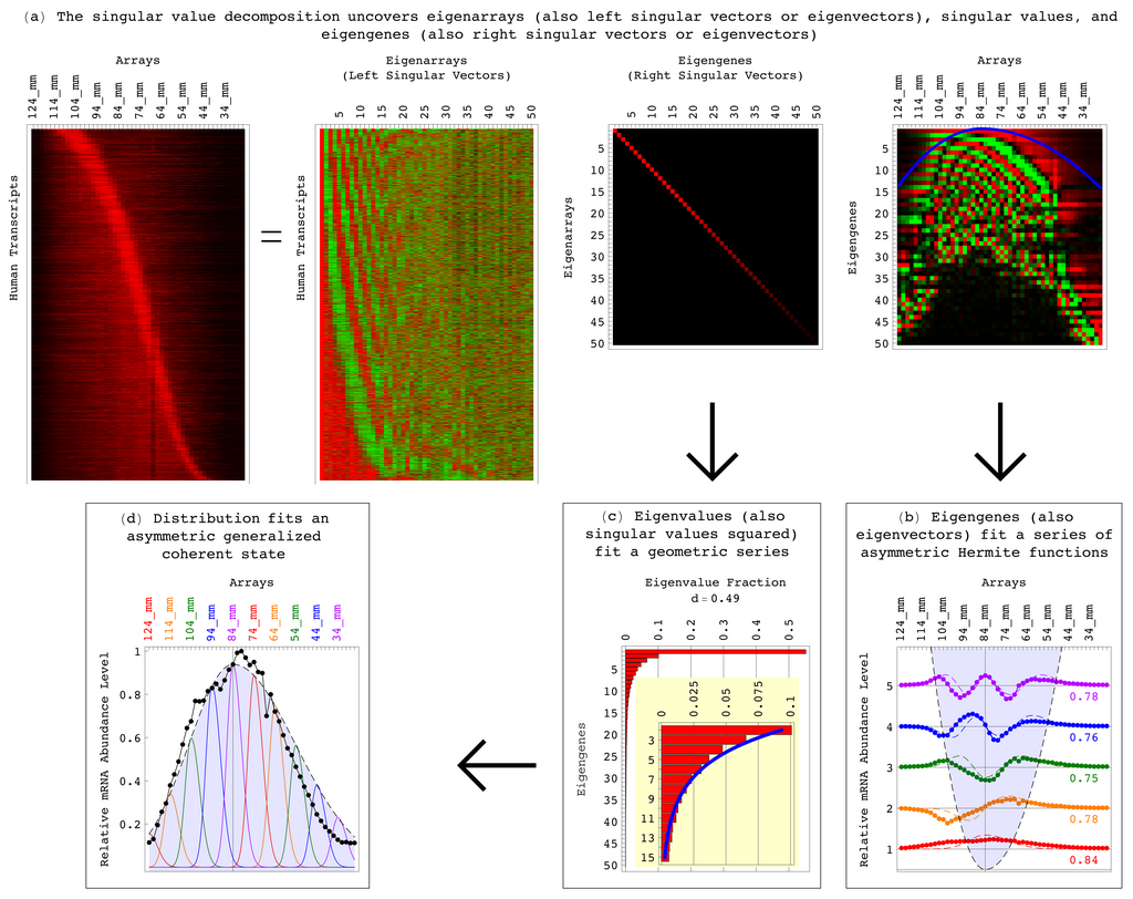
This decomposition is written as:

Here's what each part means:

• $U$ is a rotation matrix.
• $\Sigma$ (Sigma) is a diagonal matrix that scales the data. Its non-zero elements are called singular values.
• $V^T$ is another rotation matrix.

SVD tells us that any linear transformation can be broken down into a rotation, followed by a scaling along the axes, followed by another rotation. The singular values in $\Sigma$ are ordered by size, telling us how much 'stretch' happens in each direction. This is incredibly useful for data compression, noise reduction, and recommendation systems. By keeping only the largest singular values and their corresponding vectors in $U$ and $V$, we can create a close approximation of the original matrix with much less data.

Understanding these core concepts of linear algebra gives you the toolkit to understand how data is represented and manipulated inside many powerful AI algorithms.