Mastering Statistical Inference and Confidence Intervals
Sampling Distribution Logic
From One Sample to Many
So far, you've learned how to describe a single set of data using measures like the mean and standard deviation. But in statistics, we rarely care about just one sample. Our real goal is to use a sample to understand a much larger population. To do that, we need to bridge the gap between what our sample tells us and what might be true for the whole group. This bridge is built with sampling distributions.
Parameter vs. Statistic
First, let's get our terms straight. A parameter is a number that describes a characteristic of an entire population. A statistic is a number that describes a characteristic of a sample. The core idea of inference is using a statistic to estimate a parameter.
Think of it this way: a census of every person in a country would give you a parameter (the true average age). A survey of 1,000 people would give you a statistic (the sample's average age). We hope the statistic is close to the parameter, but we know it won't be perfect.
| Concept | Population (Parameter) | Sample (Statistic) |
|---|---|---|
| Mean | μ (mu) | x̄ (x-bar) |
| Proportion | p | p̂ (p-hat) |
| Standard Deviation | σ (sigma) | s |
This distinction is crucial. We almost never know the true value of a population parameter. That's why we take samples. The challenge is figuring out how much we can trust our sample statistic.
The Logic of Sampling
Imagine you want to know the true proportion of voters in a city who favor a certain candidate. The true proportion, p, is our parameter. It's impossible to ask everyone.
Instead, you take a random sample of 100 voters and find that 55 of them favor the candidate. Your sample proportion, or p̂, is 0.55. But if your friend also takes a random sample of 100 voters, they might get 52, for a p̂ of 0.52. Another friend might get 59. Each random sample will likely produce a slightly different statistic.
Now, imagine taking every possible sample of 100 voters from that city, calculating p̂ for each one, and making a histogram of all those p̂ values. This new distribution of all the sample statistics is called a sampling distribution.
A sampling distribution is the theoretical probability distribution of a statistic obtained from all possible samples of a specific size from a population.
This is a powerful idea. While we only take one sample in real life, the sampling distribution tells us how our statistic (like p̂ or x̄) would behave if we could repeat the sampling process over and over. It shows us the variability we can expect just due to random chance.
The Central Limit Theorem
Here's where things get interesting. A remarkable statistical rule, the Central Limit Theorem (CLT), tells us what shape this sampling distribution will take.
The CLT states that for a sufficiently large sample size, the sampling distribution of the sample mean (x̄) or sample proportion (p̂) will be approximately normal, regardless of the shape of the original population's distribution. This is true as long as the samples are random and independent.
The Central Limit Theorem tells us that regardless of the population’s distribution shape (whether the data is normal, skewed, or even bimodal), the sampling distribution of means will become approximately normal as the sample size increases.
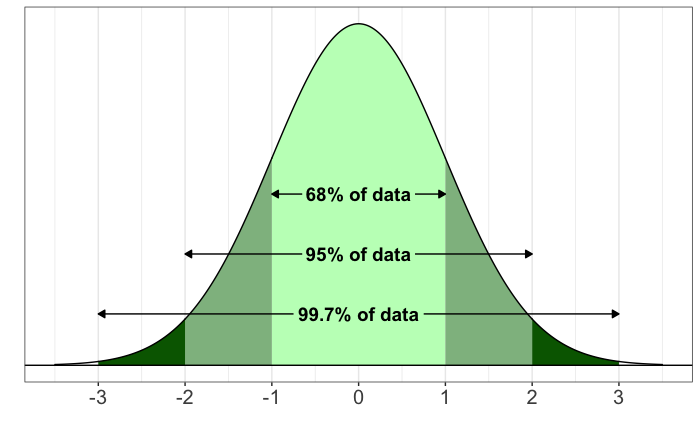
This theorem is the foundation of most inferential statistics. It lets us use the predictable properties of the normal curve to make probability statements about our sample statistics, even if we know nothing about the population's shape. As a general rule, a sample size of n ≥ 30 is considered large enough for the CLT to apply for sample means. For proportions, we'll check a different condition later.
Describing Sampling Distributions
Since sampling distributions are, well, distributions, they have a center (mean) and spread (standard deviation). The formulas for these are specific to the statistic we're measuring.
The Sample Proportion (p̂)
Let's say we're interested in proportions. The sampling distribution of p̂ has a mean and standard deviation defined as:
The Sample Mean (x̄)
Now, for sample means. The sampling distribution of x̄ has its own mean and standard deviation:
Notice a common theme? In both formulas for standard deviation, the sample size n is in the denominator. This brings us to another key idea.
The Law of Large Numbers
The Law of Large Numbers states that as the sample size increases, the sample statistic (like x̄ or p̂) will get closer and closer to the true population parameter (μ or p). The formulas we just saw show this mathematically.
Look at the standard deviation formula for x̄: . As n gets bigger, the denominator gets bigger, making the overall standard deviation smaller. A smaller standard deviation means less variability. The sample means will cluster more tightly around the true population mean. The same logic applies to proportions.
Bigger samples give better estimates because they produce statistics with less variability.
This graphic illustrates the effect of sample size. All three distributions are centered at the same true mean (μ), but as n increases, the distribution gets tighter. An x̄ from a sample of 100 is much more likely to be close to μ than an x̄ from a sample of 10.
The Conditions for Inference
These powerful ideas only work if certain conditions are met. For any inferential procedure, you must verify three things:
- Random: The data must come from a random sample or a randomized experiment. This prevents bias.
- Normal: The sampling distribution must be approximately normal. We can assume this if the population is stated to be normal, or if our sample size is large enough (the CLT).
- Independent: Individual observations must be independent. When sampling without replacement, the population must be at least 10 times larger than the sample size (the 10% condition). This ensures that taking one individual out doesn't significantly change the probability for the next.
These 'Random, Normal, Independent' conditions are the gatekeepers of statistical inference. They ensure our mathematical models are appropriate for the data. You will check them for every confidence interval and hypothesis test you perform.
Now, let's test your understanding of these foundational concepts.
A political analyst wants to know the true percentage of all registered voters in a state who support a new law. They conduct a random survey of 1,200 voters and find that 57% of them are in favor. In this context, what does the value 57% represent?
The Central Limit Theorem (CLT) is a foundational concept in statistics. What is the primary conclusion of the CLT?
Understanding how statistics vary across samples is the key that unlocks our ability to draw meaningful conclusions about the world from data.