Mastering Physics Informed Machine Learning
Physics Informed Machine Learning
Beyond Black Boxes
Standard machine learning models are powerful, but they operate as "black boxes." They learn patterns from data without any understanding of the underlying principles governing a system. For many tasks, like classifying images or predicting customer churn, this is perfectly fine. The model finds statistical correlations, and that's enough.
However, when we model physical systems—like fluid dynamics, heat transfer, or structural mechanics—this purely data-driven approach has serious limitations. A neural network trained on sensor data from a jet engine might make a prediction that violates the laws of thermodynamics. It doesn't know any better. It only knows what it has seen in its training data. If it encounters a new scenario, its predictions can become physically nonsensical.
This is the core problem: data-driven models are great interpolators but poor extrapolators, especially when physical laws are non-negotiable.
Another major hurdle is data scarcity. Gathering high-fidelity data from physical experiments or complex simulations is often expensive and time-consuming. Traditional deep learning models are data-hungry, and without a massive dataset, they struggle to generalize, often leading to overfitting. This is where the old guard of scientific computing, traditional numerical solvers like Finite Element Analysis (FEA), have historically shined. They don't need training data because they are built entirely on the mathematical equations that describe the physics.
A Hybrid Approach
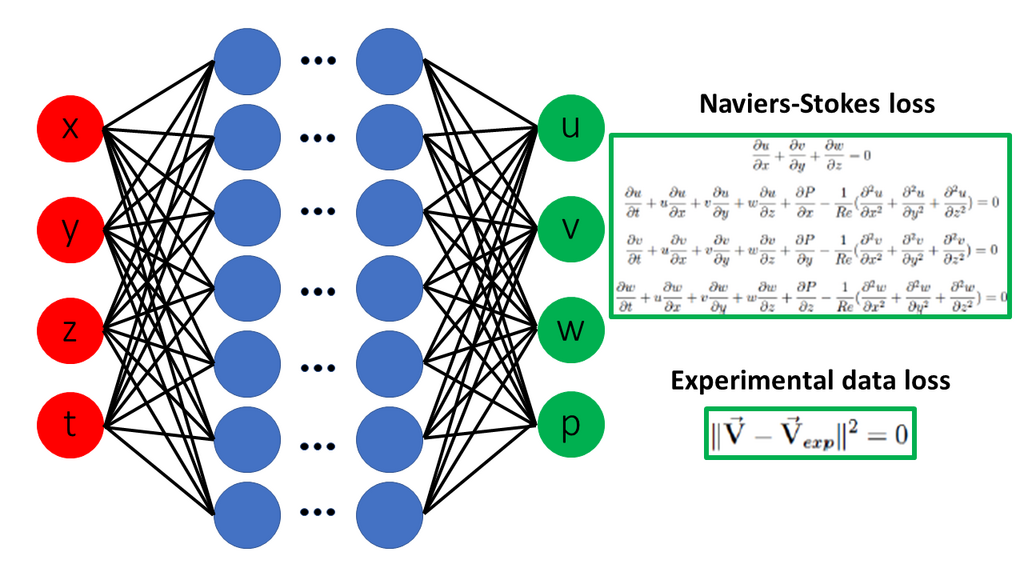
Physics-Informed Machine Learning (PIML) offers a middle ground, merging the flexibility of neural networks with the rigor of physical laws. Instead of treating the model as a black box, we treat it as a "grey box." We still use a neural network as a universal function approximator to learn from data, but we inject domain knowledge directly into the training process. This is done by modifying the loss function.
In standard supervised learning, the loss function measures the difference between the model's prediction and the true label. In PIML, we add a new component to this loss: a term that measures how well the model's output conforms to a governing physical law, typically expressed as a Partial Differential Equation (PDE).
The physics loss, , is calculated from the residual of the PDE. Let's say we have a function that is governed by a differential equation . We train a neural network to approximate . The physics loss is the mean squared error of the PDE residual, evaluated at a set of randomly sampled points in the domain (called collocation points).
This forces the network to find a solution that not only fits the available data but also obeys the known laws of physics. It acts as a powerful form of regularization, guiding the model towards physically plausible solutions, especially in regions where no training data exists.
Inductive Bias and Trade-offs
By adding the physics loss, we are introducing a strong inductive bias into the model. An inductive bias refers to the assumptions a model makes to generalize from finite training data to unseen situations. For example, a linear regression model has a bias that the underlying relationship is linear. In PIML, our bias is that the solution must adhere to specific physical laws.
This hybrid approach elegantly addresses the trade-offs between purely data-driven and theory-driven modeling. Traditional PDE solvers are precise but can be computationally slow and struggle with complex geometries or missing boundary conditions. Data-driven models are fast and flexible but require vast amounts of data and can produce physically impossible results.
| Approach | Pros | Cons |
|---|---|---|
| Data-Driven (Black Box) | Highly flexible, learns complex patterns. | Requires large datasets, can be physically inconsistent. |
| Theory-Driven (Solvers) | Physically accurate, requires no training data. | Computationally expensive, rigid, needs well-defined problems. |
| PIML (Grey Box) | Data-efficient, physically consistent, fast inference. | Requires known governing equations, can be complex to implement. |
PIML systems can learn from sparse, noisy data and still produce high-fidelity results because the underlying physics constrains the space of possible solutions. It's like trying to solve a puzzle with most of the pieces missing, but having the final picture on the box as a guide. The physical laws provide that essential guide, bridging the gaps in the data.
Physics-informed machine learning (PIML) is emerging as a potentially transformative paradigm for modeling complex biomedical systems by integrating parameterized physical laws with data-driven methods.
So, how is the physics loss actually calculated? It leverages a technique called automatic differentiation to compute the derivatives of the neural network's output with respect to its inputs. This allows us to plug the network directly into the differential equation and evaluate the residual without needing to perform numerical differentiation, which can be unstable.
This paradigm shift redefines what a loss function can represent. It's no longer just about matching labels. It's about encoding fundamental truths of the physical world into the learning process itself.
What is a primary limitation of standard 'black box' machine learning models when used to model physical systems?
How does Physics-Informed Machine Learning (PIML) primarily enforce physical laws during the training of a neural network?