Electrical circuits can get complicated, fast. A network of resistors, voltage sources, and current sources can look like a tangled mess. When you want to analyze what's happening at just one part of that circuit—say, across a specific component called the 'load'—calculating the effect of everything else can be a headache.

Luckily, we have powerful tools to simplify things. One of the most useful is Norton's theorem. It allows us to take a large, complex part of a circuit and replace it with a much simpler, equivalent circuit that behaves identically from the load's perspective.

Norton's theorem states that any linear electrical network can be replaced by a simple equivalent circuit. This isn't just an approximation; from the perspective of the load, the behavior is exactly the same. No matter how many sources and resistors are in the original circuit, we can boil it down to two key components.

This simplified circuit consists of two parts:

• Norton Current ($I_N$): An ideal current source. This is the current that would flow through the terminals of the load if they were short-circuited (connected directly together).
• Norton Resistance ($R_N$): A resistor placed in parallel with the current source. This represents the total equivalent resistance of the original circuit looking back from the load terminals, with all independent voltage sources shorted and all independent current sources opened.

This transformation is powerful because it allows us to ignore the complexity of the original circuit and focus only on how this simpler equivalent circuit affects the load we care about.

If you're familiar with Thévenin's theorem, you might see a strong similarity. Thévenin's theorem simplifies a circuit into a single voltage source ($V_{Th}$) in series with a resistor ($R_{Th}$). Norton's theorem simplifies the same circuit into a single current source ($I_N$) in parallel with a resistor ($R_N$).

These two are not just similar; they are exact equivalents of each other. This is known as source transformation. Any Thévenin equivalent circuit can be converted into a Norton equivalent circuit, and vice-versa.

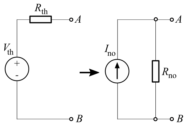
The key relationship is that the Norton resistance is identical to the Thévenin resistance. They are calculated in the same way.

The Norton current and Thévenin voltage are related by Ohm's Law:

This dual relationship makes Norton's theorem an incredibly flexible tool for circuit analysis. Sometimes it's easier to find the Thévenin equivalent, and other times the Norton equivalent is more straightforward.

Norton's theorem, like Thévenin's theorem, has its limits. It can only be applied to circuits that are linear and bilateral.

• A linear circuit is one where the output is directly proportional to the input. It's composed of elements like resistors, capacitors, and inductors, whose values don't change with voltage or current.

• A bilateral element is one that works the same way regardless of the direction of current flowing through it. Resistors are a great example.

This means you can't use Norton's theorem to simplify circuits containing non-linear components like diodes or transistors, unless you're analyzing them within a specific, linear operating range.

Understanding this concept is the first step. Next, we'll walk through the process of calculating the Norton equivalent for a real circuit.