So far, you've likely used transfer functions to model systems. They're powerful tools, giving a direct relationship between a single input and a single output. A system is treated like a black box; you put something in, and the transfer function tells you what comes out. This works well for many simple systems.

But what about more complex scenarios? Consider a modern drone. It has multiple inputs (the thrust of each of its four motors) and multiple outputs (its position, orientation, and velocity in 3D space). This is a Multi-Input Multi-Output (MIMO) system. Trying to describe it with a single transfer function is cumbersome and often impractical. More importantly, a transfer function doesn't tell us what's happening inside the system. It hides the internal workings.

State-space representation offers a more detailed and flexible approach. Instead of just modeling the input-output relationship, it models the internal state of the system itself. This allows us to handle complex MIMO systems and gives us a clearer picture of the system's dynamics.

The core of this method is the concept of state variables. A set of state variables is the smallest possible group of variables that, along with the system's inputs, can completely describe the future behavior of the system. Think of them as a snapshot of the system's internal energy-storing elements at a specific moment.

Let's take a classic mechanical example: a mass-spring-damper system. The energy in this system is stored in two ways: as potential energy in the compressed or stretched spring, and as kinetic energy in the moving mass. The state of this system can be fully described by two variables: the position of the mass, $y(t)$, and the velocity of the mass, $\dot{y}(t)$. Knowing just these two values at any given time, plus any external force being applied, is enough to predict the mass's future motion.

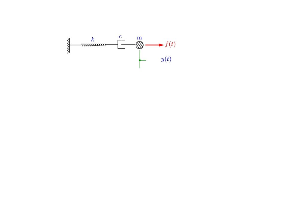
We group these state variables into a single column vector called the state vector, denoted as $\mathbf{x}$. For our example, the state vector would be:

State-space models are universally expressed with a pair of equations. These equations describe how the state vector and the output evolve over time.

These four matrices, A, B, C, and D, define the entire system. Let's break down what each one does:

• A: The System Matrix. This matrix describes the internal dynamics of the system. If there were no external inputs ($\mathbf{u}=0$), the states would evolve according to $\dot{\mathbf{x}} = A\mathbf{x}$. It shows how the state variables are coupled and how they change on their own.

• B: The Input Matrix. This matrix determines how the inputs affect the state variables. It acts as a bridge, mapping the external forces or signals in $\mathbf{u}$ to changes in the internal state $\mathbf{x}$.

• C: The Output Matrix. Often, we can't directly measure every state variable. The output matrix defines what we can measure. It selects or combines state variables to form the output vector $\mathbf{y}$.

• D: The Feedforward Matrix. This matrix represents a direct path from the input to the output, bypassing the system's internal dynamics. In many physical systems, especially mechanical ones, this matrix is zero, meaning the input must first affect the state before it can influence the output.

Let's convert our mass-spring-damper system into state-space form. Newton's second law gives us the governing differential equation, where $f(t)$ is the input force:

To get this into state-space form, which uses first-order equations, we first isolate the highest derivative:

Now, we define our state variables, as we did before: $x_1 = y$ and $x_2 = \dot{y}$. We need to find expressions for their derivatives, $\dot{x}_1$ and $\dot{x}_2$. The first one is simple:

For the second, we use our rearranged differential equation:

We now have our set of first-order differential equations. We can write them in matrix form $\dot{\mathbf{x}} = A\mathbf{x} + B\mathbf{u}$:

Finally, let's say we're interested in measuring the position of the mass as our output. This means our output equation is simply $y_{out} = x_1$. In matrix form, $\mathbf{y} = C\mathbf{x} + D\mathbf{u}$, this becomes:

And there it is. We've successfully modeled a physical system using the A, B, C, and D matrices. This compact representation is not just neat; it's the foundation for modern control theory, enabling analysis and design for systems far more complex than this simple example.