Mastering Computer Vision Edge Detection
Image Gradients and Calculus
Images as Functions
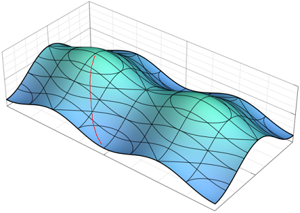
To a computer, an image is just a grid of numbers. Each number represents the intensity, or brightness, of a pixel at a specific location. We can think of this grid as a function, usually written as , where are the pixel coordinates and the function's output is the intensity value at that point.
Unlike the smooth, continuous functions you might remember from a calculus class, an image is a discrete function. The inputs are integers, not continuous variables, and the function is only defined at these specific grid points. This distinction is key. To find where edges are, we need to find where the intensity changes rapidly. This means we need a way to measure the rate of change, or slope, on our discrete grid.
Finding Change with Derivatives
In calculus, the tool for measuring change is the derivative. Since our image function has two variables, we need to use partial derivatives—one to measure the rate of change horizontally (along the x-axis) and another to measure it vertically (along the y-axis).
The gradient is a fancy word for derivative, or the rate of change of a function.
Because our pixel grid is discrete, we can't use the standard limit-based definition of a derivative. Instead, we approximate it. The simplest way is with a approximation. To find the change in the x-direction at a pixel, we just subtract the intensity of the pixel to its left from the pixel to its right. The same logic applies to the y-direction.
The Gradient Vector
By combining these two partial derivatives, we get the gradient vector, denoted as . This vector is powerful because it tells us two things at once: its direction points towards the steepest increase in intensity, and its magnitude tells us how steep that increase is. A large magnitude signifies a sharp change in intensity—an edge. A small magnitude means the area is flat, with little change.
Let's calculate the gradient for the central pixel of a 3x3 image patch. Here are the intensity values:
| y=0 | y=1 | y=2 | |
|---|---|---|---|
| x=0 | 10 | 10 | 90 |
| x=1 | 10 | 50 | 90 |
| x=2 | 10 | 90 | 90 |
Our target is the central pixel , which has an intensity of 50.
First, the horizontal change, :
Next, the vertical change, :
So, the gradient vector at pixel is .
Edge Strength and Direction
The gradient vector is useful, but for edge detection, we usually need two scalar values: the gradient magnitude and its direction.
The magnitude tells us the strength of the edge. It's calculated just like the hypotenuse of a right-angled triangle, using the Pythagorean theorem. A larger magnitude means a more prominent edge.
The direction tells us the orientation of the edge. It's the angle of the gradient vector, which can be found using basic trigonometry. The edge itself is always perpendicular to the gradient direction.
By calculating the gradient magnitude for every pixel, we can generate a new image, called a gradient map, where high-intensity values correspond to strong edges in the original image. This map is the foundation for many edge detection algorithms.
In the context of digital images, what does the function typically represent?
Why must we use a finite difference approximation instead of a standard calculus derivative to measure intensity changes in an image?