We begin with the fundamental force that governs the interaction between stationary charges: Coulomb's Law. You're likely familiar with its scalar form, which tells us the magnitude of the force. However, to fully describe the interaction, we need to consider its direction. This requires the vector form of the law.

Let's say we have two point charges, $q_1$ and $q_2$, located at positions given by vectors $\vec{r_1}$ and $\vec{r_2}$. The force exerted by $q_1$ on $q_2$, denoted by $\vec{F}_{12}$, is not just a number; it's a vector pointing along the line connecting the two charges.

The unit vector $\hat{r}_{12}$ is defined as $\frac{\vec{r}_2 - \vec{r}_1}{|\vec{r}_2 - \vec{r}_1|}$. This ensures the force acts along the line joining the charges. If $q_1$ and $q_2$ have the same sign, the force is repulsive (pointing away). If they have opposite signs, it's attractive (pointing inwards).

What happens when there are more than two charges? The total force on any single charge is simply the vector sum of the forces exerted on it by all other charges. This is the Principle of Superposition.

Instead of calculating forces between pairs of charges, it's often more useful to think about an electric field, $\vec{E}$. A charge creates an electric field in the space around it, and any other charge placed in this field experiences a force, $\vec{F} = q\vec{E}$.

To visualise this field, we use the concept of electric flux, $\Phi_E$. Imagine the electric field lines as streams of water. Flux is a measure of how many of these field lines pass through a given surface. For a uniform field $\vec{E}$ passing through a flat area $\vec{A}$, the flux is $\Phi_E = \vec{E} \cdot \vec{A}$.

This leads to one of the most powerful tools in electrostatics: Gauss's Law. It connects the electric flux through a closed surface (called a Gaussian surface) to the total charge enclosed within that surface.

The magic of Gauss's Law is that if we choose our Gaussian surface cleverly, we can calculate the electric field for symmetric charge distributions much more easily than by using Coulomb's Law and superposition. Let's examine the three key applications for your board exams.

1. Infinitely long straight wire: We use a cylindrical Gaussian surface of radius $r$ and length $l$, coaxial with the wire. The electric field points radially outwards, so flux only passes through the curved surface, not the flat caps. The result is $E = \frac{\lambda}{2\pi\epsilon_0 r}$, where $\lambda$ is the linear charge density (charge per unit length).

2. Uniformly charged infinite plane sheet: Here, we use a small cylindrical 'pillbox' that pierces the sheet. The electric field is uniform and perpendicular to the sheet. Flux only passes through the two flat caps of the pillbox. This gives a constant electric field, $E = \frac{\sigma}{2\epsilon_0}$, where $\sigma$ is the surface charge density. Notice the field doesn't depend on the distance from the sheet!

3. Uniformly charged thin spherical shell: We use a spherical Gaussian surface. For a point outside the shell ($r > R$), the shell behaves as if all its charge $Q$ were concentrated at its centre, giving $E = \frac{1}{4\pi\epsilon_0} \frac{Q}{r^2}$. For a point inside the shell ($r < R$), the enclosed charge is zero. Therefore, the electric field inside a uniformly charged spherical shell is zero.

The electric field tells us about the force on a charge. The electric potential, $V$, tells us about the potential energy. Electric potential at a point is the work done per unit charge in bringing a positive test charge from infinity to that point.

The relationship between field and potential is crucial: the electric field points in the direction of the steepest decrease in potential. Mathematically, $E = -\frac{dV}{dr}$.

For a single point charge $Q$, the potential at a distance $r$ is:

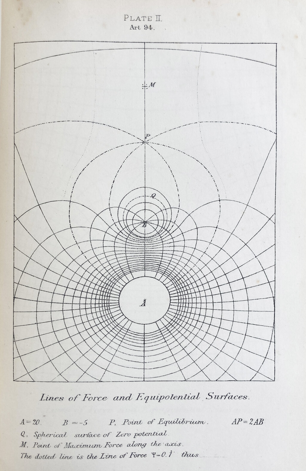
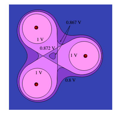
An equipotential surface is a surface where the electric potential is the same at every point. No work is done in moving a charge along an equipotential surface. A key property is that electric field lines are always perpendicular to equipotential surfaces.

Now consider an electric dipole, which consists of two equal and opposite charges, $+q$ and $-q$, separated by a small distance $2a$. The potential due to a dipole at a point far away is more complex, depending on both the distance $r$ from the center of the dipole and the angle $\theta$ with respect to the dipole axis.

When a dipole is placed in a uniform external electric field $\vec{E}$, it experiences a torque that tries to align it with the field. The torque is given by $\vec{\tau} = \vec{p} \times \vec{E}$, and the potential energy of the dipole is $U = -\vec{p} \cdot \vec{E}$.

A capacitor is a device designed to store electrical energy. It typically consists of two conductors separated by an insulator. The ability of a capacitor to store charge is measured by its capacitance, $C$, defined as the ratio of the charge on one conductor to the potential difference between them: $C = Q/V$.

The most common type is the parallel plate capacitor, consisting of two parallel conducting plates, each of area $A$, separated by a distance $d$.

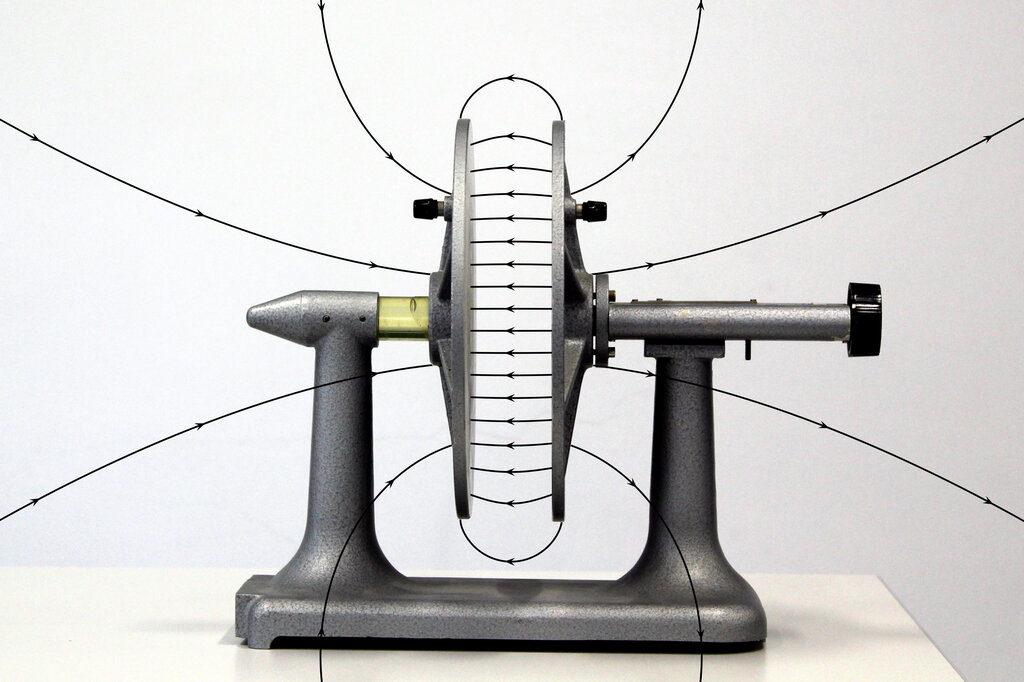
What happens if we insert an insulating material, called a dielectric, between the plates? The molecules of the dielectric polarise in the presence of the electric field. This creates an internal electric field within the dielectric that opposes the external field, reducing the overall field strength.

Since the potential difference $V=Ed$ is reduced for the same charge $Q$, the capacitance $C=Q/V$ increases. The new capacitance is given by:

The work done to charge a capacitor is stored as potential energy in the electric field between the plates. This stored energy can be expressed in several ways:

In circuits, capacitors can be combined in series or parallel. For capacitors in series, the equivalent capacitance $C_{eq}$ is found by $\frac{1}{C_{eq}} = \frac{1}{C_1} + \frac{1}{C_2} + \dots$. For capacitors in parallel, it's a simple sum: $C_{eq} = C_1 + C_2 + \dots$.

Ready to test your understanding? Let's work through some questions.

These principles of electrostatics form the bedrock for understanding electric circuits, magnetism, and ultimately, the behaviour of light itself.