Simple gradient descent is a reliable starting point for training a neural network, but it's like hiking down a mountain in the fog with tiny, uniform steps. It moves in the direction of the steepest descent, but it can be painfully slow on flat plateaus and can get trapped in local minima. Even worse, it struggles with saddle points—areas that look like a minimum in one direction but a maximum in another. To train deep networks effectively, we need more sophisticated navigation tools.

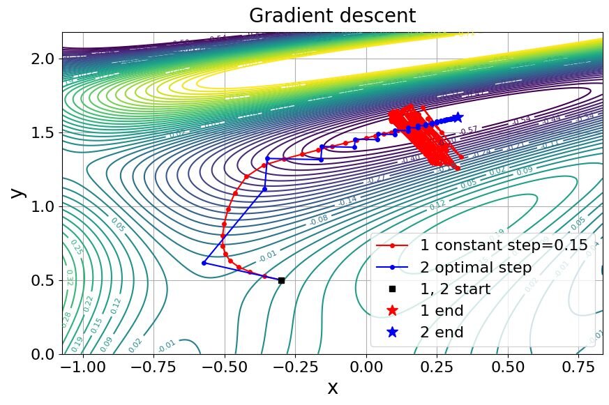
One of the first upgrades is Momentum. Imagine a ball rolling down a hill. Instead of just looking at the current slope, Momentum adds a fraction of the previous update step to the current one. This helps the ball build up speed on steep descents and coast through flat areas or shallow local minima. It accelerates learning and dampens oscillations.

Then there's RMSprop (Root Mean Square Propagation). This optimizer adapts the learning rate for each parameter individually. It keeps a moving average of the squared gradients for each weight. If a weight's gradients are consistently large, RMSprop shrinks its effective learning rate. If they're small, it boosts the learning rate. This is incredibly useful for navigating ravines and other complex loss landscapes where different parameters need different step sizes.

Adam, which stands for Adaptive Moment Estimation, combines the best of both worlds. It uses the moving average of the gradient (like Momentum) and the moving average of the squared gradient (like RMSprop). This gives it both the acceleration of momentum and the adaptive learning rates of RMSprop, making it a powerful and popular default choice for many deep learning tasks.

Every model we train performs a balancing act. It's called the bias-variance tradeoff.

Bias is the error from a model's simplifying assumptions. A model with high bias pays little attention to the training data and oversimplifies the true relationship. This leads to underfitting. An example would be trying to fit a straight line to data that follows a clear curve.

Variance is the error from a model's sensitivity to small fluctuations in the training data. A model with high variance pays too much attention to the training data, capturing not just the underlying pattern but also the noise. This leads to overfitting. It performs brilliantly on the data it was trained on but fails to generalize to new, unseen data.

As a model's complexity increases (e.g., more layers or neurons), its bias decreases, but its variance increases. The goal isn't to eliminate one or the other, but to find the sweet spot where the total error is minimized. This is where regularization comes in.

Regularization techniques are designed to reduce high variance without significantly increasing bias. They impose a penalty on complexity, guiding the model toward simpler, more generalizable solutions.

L2 Regularization, also known as weight decay, adds a term to the loss function that penalizes large weight values. It's calculated as the sum of the squares of all the weights in the network. This encourages the model to use all of its inputs to make decisions, rather than relying heavily on just a few. The result is a 'flatter' weight distribution and a model that is less sensitive to individual data points.

Dropout is a brilliantly simple yet effective technique. During each training step, it randomly sets a fraction of neuron activations to zero. This forces the network to learn redundant representations and prevents neurons from co-adapting too much. It's like training a committee of experts where, at any given time, you don't know which experts will show up. Each member has to be competent on their own, making the whole committee more robust.

Finally, there's Batch Normalization. This technique normalizes the output of a previous activation layer by subtracting the batch mean and dividing by the batch standard deviation. It addresses a problem called internal covariate shift, where the distribution of each layer's inputs changes during training as the parameters of the previous layers change. By stabilizing these distributions, Batch Norm allows for much higher learning rates, speeds up training significantly, and provides a slight regularization effect. It's often placed between a linear layer and a non-linear activation function.

Building a high-performance model isn't just about choosing the right architecture and optimizer; it's also about fine-tuning the details.

Hyperparameter Tuning is the process of finding the optimal values for parameters that aren't learned during training, like the learning rate, the dropout rate, or the strength of L2 regularization. Common strategies include Grid Search (exhaustively trying all combinations), Random Search (sampling random combinations, often more efficient), and more advanced methods like Bayesian Optimization.

To ensure all this complex machinery works, we need to verify our implementation. Gradient Checking is a crucial debugging technique. It involves numerically approximating the gradients and comparing them to the gradients calculated by backpropagation. If the values are far apart, there's a bug in your backpropagation code. It's computationally expensive, so you only run it on a small subset of data during development, and you turn it off for actual training.

These optimization and regularization methods are the workhorses of modern deep learning. They manage the delicate balance between fitting our data and generalizing to new problems, enabling us to build and train the incredibly deep and complex networks that power today's AI.