Many natural phenomena, from the heights of people to the measurement errors in an experiment, tend to follow a specific pattern. When you plot this data, it often forms a symmetrical, bell-shaped curve. This pattern is known as the normal distribution, and it's a cornerstone of statistics because it describes how data is spread around a central value.

The curve is densest in the middle and less dense at the tails. This means that values close to the average are very likely, while values far from the average are rare. The curve is perfectly symmetrical, so the right side is a mirror image of the left. A key feature of the normal distribution is that the mean, median, and mode are all the same and are located at the center.

A normal distribution is defined by just two parameters: the mean (represented by the Greek letter $\mu$, or mu) and the standard deviation (represented by $\sigma$, or sigma).

The mean (μ) is the central point of the distribution. It determines the location of the peak of the bell curve. If you change the mean, the entire curve shifts to the left or right on the graph.

The standard deviation (σ) controls the spread or width of the curve. A smaller standard deviation indicates that the data points are tightly clustered around the mean, resulting in a tall and narrow curve. A larger standard deviation means the data is more spread out, creating a shorter and wider curve.

By knowing just these two values, you can understand the entire distribution of your data, assuming it's normally distributed.

For any normal distribution, there's a handy rule of thumb for understanding how the data is spread out. It's called the Empirical Rule, or the 68-95-99.7 rule. It provides a quick way to know the percentage of data that falls within a certain number of standard deviations from the mean.

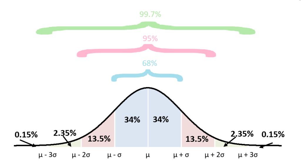
Here's the breakdown:

• Approximately 68% of the data falls within one standard deviation of the mean. This means between $(\mu - \sigma)$ and $(\mu + \sigma)$.

• Approximately 95% of the data falls within two standard deviations of the mean, so between $(\mu - 2\sigma)$ and $(\mu + 2\sigma)$.

• Approximately 99.7% of the data falls within three standard deviations of the mean, between $(\mu - 3\sigma)$ and $(\mu + 3\sigma)$.

This rule tells us that nearly all values in a normal distribution lie within three standard deviations of the mean. Values outside this range are very rare.

The Empirical Rule is powerful because it allows us to quickly estimate probabilities and identify common versus unusual data points without complex calculations, as long as the data follows a normal distribution.