In machine learning, training a model is an act of optimization. We have a loss function that tells us how badly the model is performing, and our goal is to adjust the model's parameters (its weights and biases) to make that loss as small as possible. The process is often compared to a hiker trying to find the lowest point in a valley. The hiker's position represents the current parameter values, and the altitude is the loss.

This landscape of loss values is called the loss surface. For simple problems, this surface is a smooth, predictable bowl. This is known as a convex surface. No matter where you start, if you always walk downhill, you'll eventually reach the single lowest point, the global minimum. It’s an ideal scenario for optimization.

Deep learning models, with their millions or even billions of parameters, create astronomically complex, high-dimensional loss surfaces. These are non-convex, meaning they are riddled with numerous valleys (local minima), hills, and plateaus. Navigating this terrain is the central challenge of training deep neural networks. An algorithm might find a valley that seems like the bottom, a local minimum, but a much deeper valley, the global minimum, could exist elsewhere on the surface. Getting stuck in a suboptimal valley means the model won't perform as well as it could.

To navigate this landscape effectively, we need more than just the direction of the slope, which is given by the gradient. We also need to understand the surface's curvature, or how it bends. This is where the Hessian matrix comes in. The Hessian is a matrix of second-order partial derivatives of the loss function. While the gradient (first-order derivative) tells us the direction of steepest descent, the Hessian (second-order derivative) tells us how the gradient will change as we move.

A positive curvature (like the inside of a bowl) indicates we're near a minimum. A negative curvature (like the top of a hill) signals a maximum. This information allows for more sophisticated optimization algorithms than simple gradient descent. For instance, Newton's method uses the Hessian to take more direct, intelligent steps towards a minimum, like calculating the perfect arc to land at the bottom of the valley instead of taking many small steps.

For a long time, it was believed that local minima were the biggest obstacle in training neural networks. However, research has shown that in the high-dimensional spaces of deep learning, saddle points are a much more common and troublesome feature. A saddle point is a location that is a minimum along some dimensions but a maximum along others. Imagine the center of a horse's saddle: it curves up from front to back but down from side to side.

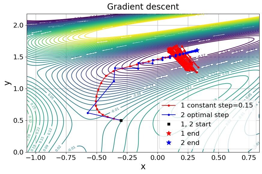
At a saddle point, the gradient is zero, just like at a minimum or maximum. A simple gradient descent algorithm might get stuck there, oscillating back and forth, because it sees no clear downhill direction. The loss stops improving, and training stalls. Fortunately, algorithms with momentum or adaptive learning rates are often better at "rolling through" these saddle points. The curvature information from the Hessian would immediately reveal that a point is a saddle (it has both positive and negative curvature), but since we can't usually compute it, we rely on algorithmic tricks to escape.

The overall 'smoothness' of the loss landscape also plays a huge role in optimization stability. A 'bumpy' or 'jagged' loss surface, where the gradient changes sharply and erratically, can cause the optimizer to jump around wildly, failing to converge. A 'smooth' surface allows for a more stable and predictable descent. The choice of loss function and even the model's architecture can influence this smoothness. Some activation functions, like ReLU, can create sharp corners in the landscape, while others produce smoother surfaces.

Finally, where you start your hike matters. Initialization, the process of setting the initial weights of the model, is equivalent to dropping the hiker at a random spot on the loss landscape. A good initialization strategy can place you in a 'good' region of the landscape, one with a smooth path down to a deep valley. A bad initialization might start you in a flat plateau or on a steep cliff, making the optimizer's job much harder. This interaction between starting point and landscape geometry is a key factor in whether a model trains successfully.

Time to check what you've learned.

Understanding the shape of your loss function is crucial for diagnosing training problems and choosing the right optimization strategy.