Machine Learning for Personalization
Evaluation and Testing
Measuring What Matters
You've built sophisticated models, from two-tower architectures to LLM-powered rankers. Now comes the hard part: proving they actually work. In a production environment, simply predicting a user's next click isn't enough. We need to measure if our recommendations are truly useful, engaging, and profitable. This means moving beyond offline accuracy and embracing metrics designed for ranking and long-term user satisfaction.
The most common mistake is to treat recommendation as a classification problem. A user doesn't just want one 'correct' item; they want a high-quality, ordered list. Our evaluation must reflect this. We care more about getting a great item in the top 3 positions than in position 30. This is where ranking-aware metrics come in.
Let's start with Recall@K, which answers a simple question: Out of all the items a user actually liked, what fraction did we show in our top K recommendations? If a user watched 10 movies last month and our model recommended 4 of them in the top 20, our Recall@20 is 4/10, or 40%. It's a great metric for the candidate generation stage, where our goal is to not miss anything potentially relevant.
Another key metric is Mean Reciprocal Rank (MRR). For each user, we look at the rank of the first relevant item we recommended. If the first correct item is at position 3, the reciprocal rank is 1/3. If it's at position 1, the rank is 1/1. MRR is simply the average of these reciprocal ranks across all users. It heavily rewards models that place a correct item right at the top.
Position Matters Most
While Recall@K and MRR are useful, the gold standard for ranking quality is Normalized Discounted Cumulative Gain, or NDCG. It's a bit more complex, but it captures two crucial ideas: relevant items are better than irrelevant ones, and relevant items shown earlier in a list are more valuable than those shown later.
It works by assigning a relevance score to each recommended item (e.g., 0 for ignored, 1 for clicked, 5 for purchased). Then, it calculates the 'gain' from each item and 'discounts' that gain logarithmically based on its position. An item at position 1 gets full gain; an item at position 10 gets much less. Finally, it normalizes this score by dividing it by the score of a hypothetical perfect ranking. This brings the final value between 0 and 1, making it easy to compare across different models or user queries.
But even a perfect NDCG score can be misleading. A model could achieve a high score by only recommending items from a user's favorite artist or brand. This creates a 'filter bubble,' where the user is never exposed to new things. To combat this, we also measure serendipity, diversity, and novelty. These metrics quantify how surprising, varied, and new our recommendations are, ensuring we're expanding a user's horizons, not just reinforcing their existing tastes.
| Metric | Question it Answers | Best For... |
|---|---|---|
| Recall@K | Did we find most of the good stuff? | Candidate Generation |
| MRR | How quickly did we find the first good item? | Search, Known-Item Tasks |
| NDCG | Is the whole ranked list high-quality? | Ranking & Re-ranking |
| Diversity | How different are the items from each other? | Preventing Monotony |
| Novelty | How unknown are the recommended items to the user? | Discovery & Growth |
From Offline to Online
All the metrics we've discussed so far are calculated offline, using historical data. This is fast and cheap, but it's not the real world. Offline data is tainted by presentation bias: we only know how users reacted to what our old model showed them. We have no idea how they would have reacted to the things we didn't show them.
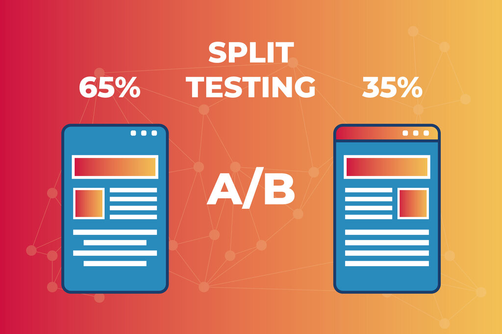
This is the fundamental gap between offline evaluation and online A/B testing. An online test involves splitting live traffic, showing a control group (A) the existing model and a treatment group (B) our new model. We can then measure the true impact on business KPIs like user retention, session length, or lifetime value. A model with a slightly lower offline NDCG might win an A/B test if it generates more novel recommendations that keep users coming back over weeks and months.
A 0.5% lift in an offline metric is an interesting result. A 0.5% lift in long-term user retention in an A/B test is a business victory.
But A/B tests are slow and expensive. We can't test every single idea. A more advanced technique, known as counterfactual evaluation, tries to bridge this gap. Using methods like Inverse Propensity Scoring (IPS), we can re-weigh our historical data to estimate what would have happened if we had shown a different set of recommendations. IPS works by giving more weight to interactions that were unlikely to happen under the old system. For example, if a user clicked on an item that was ranked at position 50, that event gets a huge weight because it signals a very strong preference that overcame a bad ranking.
Why is treating a recommendation problem as a simple classification problem (i.e., just measuring accuracy) often misleading?
A user has purchased 5 specific items in the past. In a list of top 20 recommendations, your model successfully includes 2 of those 5 items. What is the Recall@20 for this user?
By combining strong offline ranking metrics, an awareness of novelty, and a robust online testing framework, you can ensure your recommendation system doesn't just score well on a leaderboard but drives meaningful, long-term value.