Linear Algebra in DBMS
Algebraic Relational Mapping
Databases Meet Linear Algebra
At its core, a relational database organizes information into tables, which are structured collections of rows and columns. A row, or tuple, represents a single record, while a column, or attribute, represents a specific property of that record. This structure might seem familiar to anyone who has worked with spreadsheets. It's also strikingly similar to a fundamental concept in mathematics: the matrix.
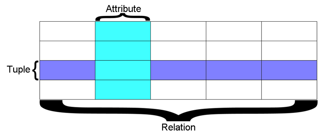
We can formally map a database relation to a matrix. If a relation has tuples and attributes, we can represent it as an matrix, let's call it . Each row in the matrix corresponds to a tuple, and each column corresponds to an attribute. This isn't just a neat visual trick; it's the foundation for applying the powerful tools of linear algebra directly to data stored in a database.
Thinking of a database table as a matrix opens up a new way to query and manipulate data.
This bridge between databases and mathematics is formalized in a framework known as Relational Matrix Algebra (RMA). RMA allows us to perform matrix operations on relations without first having to export the data into a specialized math program. The operations happen right within the database system, blending the worlds of data management and algebraic computation.
SQL as Matrix Operations
The real power of this perspective becomes clear when we translate common SQL commands into matrix operations. Two of the most fundamental SQL clauses, SELECT (for choosing columns) and WHERE (for filtering rows), have direct counterparts in matrix algebra.
Let's consider a simple table of employee data:
| EmployeeID | Department | Salary | YearsOfService |
|---|---|---|---|
| 101 | Sales | 75000 | 5 |
| 102 | HR | 62000 | 2 |
| 103 | Sales | 81000 | 8 |
| 104 | Engineering | 95000 | 4 |
An SQL query to get the Salary and YearsOfService for all employees looks like this:
SELECT Salary, YearsOfService FROM Employees;
In matrix terms, this is equivalent to column-slicing. We are extracting specific columns from our matrix. If our original matrix represents the whole table, this operation creates a new matrix containing only the 3rd and 4th columns.
Now, let's filter for employees in the 'Sales' department:
SELECT * FROM Employees WHERE Department = 'Sales';
This corresponds to row-masking. We create a mask—a vector that has a 1 for rows that meet the condition and a 0 for those that don't. We then apply this mask to select the desired rows. In our example, the mask would be , selecting the first and third rows of the matrix.
Keeping Things in Context
A raw matrix of numbers loses important information. What does each column represent? Which employee does each row correspond to? To make our matrix operations useful in a database context, we must maintain this contextual metadata. This means keeping track of column headers (attributes) and row identities (like a primary key).
When we transform a relation into a matrix, we store the column names separately. When we transform it back into a relation that can be queried with SQL, we re-attach these headers. This ensures that the result of a matrix multiplication or addition is not just a grid of numbers, but a meaningful table with queryable columns and identifiable rows.
This approach is especially efficient in databases that use a architecture. Instead of storing data row by row, these systems store it column by column. This layout is naturally suited for matrix operations, as fetching all the data for a few columns (a common task in analytics) is incredibly fast. Row-based stores, while excellent for transactional tasks like updating a single customer record, are less efficient for this kind of column-centric algebraic work.
By mapping relational tables to matrices, we create a powerful synthesis. We can leverage the speed and mathematical rigor of linear algebra for complex analytics while retaining the structured, queryable nature of a relational database.