In statistics, many things in the real world follow a specific pattern called a normal distribution. Think about the heights of adults, test scores, or even the daily returns of a stock. Most values cluster around the average, and extreme values, both high and low, become less and less common. When you plot this pattern, it forms a symmetrical, bell-shaped curve.

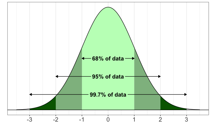
This concept is crucial in econometrics, especially when we build regression models. A common misconception is that our variables, the predictors ($X$) and the outcome ($Y$), must be normally distributed. That's not actually the case. What we really care about are the residuals, or the errors our model makes.

Imagine trying to predict house prices. Your model makes a guess for each house. The residual is simply the difference between the actual selling price and your model's prediction. A positive residual means the model underestimated the price; a negative one means it overestimated.

The Ordinary Least Squares (OLS) method, the workhorse of regression analysis, has a set of assumptions that must be met for its results to be reliable. One of the most important is that the model's residuals are normally distributed.

Why? Because this assumption is the foundation for all the statistical tests we perform after running a regression. If we want to know whether a variable has a statistically significant effect on the outcome, we use t-tests and look at p-values. If we want to create a range of likely values for our coefficients, we build confidence intervals. All of these tools rely on the math of the normal distribution.

When the errors follow a bell curve, it means that our model is making small errors much more often than large ones, and it's not systematically over- or under-predicting in a skewed way. The errors are random and centered around zero.

What happens if the residuals are not normally distributed? This is where things get tricky. The good news is that your coefficient estimates from OLS are still unbiased. This means that, on average, they are correct. Your model's prediction for the relationship between $X$ and $Y$ isn't systematically wrong.

The bad news is that the formulas we use to calculate the standard errors of those coefficients are no longer correct. This is a major problem. Without accurate standard errors, we can't conduct valid hypothesis tests. Your t-statistics will be wrong, your p-values will be misleading, and your confidence intervals will be unreliable. You might conclude a variable is significant when it isn't, or vice-versa.

Since this assumption is so important, we need ways to check it. We don't need the residuals to be perfectly normal, but they should be close. There are formal statistical tests for this, but a simple visual inspection is often the first and most useful step.

One common method is to create a histogram of the residuals. If the normality assumption holds, the histogram should look roughly like a bell curve, centered around zero.

Another popular visual tool is a Q-Q plot (quantile-quantile plot), which compares the quantiles of your residuals to the quantiles of a theoretical normal distribution. If the residuals are normal, the points on the plot will fall roughly along a straight diagonal line.

Understanding and checking this assumption is a fundamental part of building a trustworthy econometric model.