In math, some quantities can be described with a single number. Your height, for example, is just one value. But what if you need to give someone directions? You can't just say "go 5 miles." You need to specify a direction: "go 5 miles northeast."

This combination of magnitude (size or length) and direction is what we call a vector. Vectors are often used to represent things like displacement, velocity, or force. In linear algebra, we represent them as lists of numbers, typically arranged in a column.

Once we have vectors, we can perform operations on them. The two most basic operations are addition and scalar multiplication.

Vector Addition is like following two sets of directions back-to-back. If you walk 3 blocks east and 2 blocks north, and then you walk 1 block east and 4 blocks north, where do you end up? You simply add the corresponding components. Your total trip is 4 blocks east and 6 blocks north.

Mathematically, it looks like this:

Visually, we can think of this as placing the tail of the second vector at the tip of the first one. The resulting vector goes from the starting point of the first to the end point of the second.

Scalar Multiplication involves stretching or shrinking a vector. A "scalar" is just a regular number (not a vector). If you multiply a vector by a scalar, you multiply each of its components by that number. For instance, multiplying our original vector by 2 doubles its length but keeps its direction.

If you multiply by a negative scalar, you reverse the vector's direction. Multiplying by -1 gives you a vector of the same length pointing the opposite way.

If a vector is a list of numbers, a matrix is a grid of numbers, arranged in rows and columns. You can think of it like a spreadsheet. We describe the size of a matrix by its rows and columns. A matrix with 2 rows and 3 columns is a $2 \times 3$ matrix.

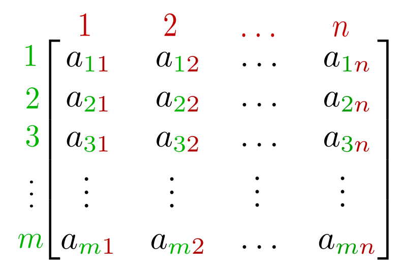
Just like with vectors, we can add matrices. The rule is simple: you can only add matrices that have the exact same dimensions. The addition happens element-wise, meaning you add the numbers in the same positions.

Matrix multiplication is different. It’s not a simple element-by-element operation. There's a key rule: to multiply matrix A by matrix B, the number of columns in A must equal the number of rows in B.

If you multiply an $m \times n$ matrix by an $n \times p$ matrix, the result will be an $m \times p$ matrix. The "inner" dimensions ($n$) must match, and the "outer" dimensions ($m$ and $p$) define the size of the result.

To find the value for a specific cell in the resulting matrix, say in the first row and first column, you multiply each element of the first row of the first matrix by the corresponding element of the first column of the second matrix, and then add up the products. This is also known as the dot product.

Look at the top-left element of the result: $ae+bg$. It comes from the first row of the first matrix (a, b) and the first column of the second matrix (e, g). The same pattern applies to all the other elements. This operation might seem strange at first, but it’s fundamental to how linear algebra is used to solve complex problems.

Let's review these new concepts before we move on.

Now, test your understanding of these operations.

Vectors and matrices are the basic building blocks of linear algebra. Mastering these definitions and operations is the first step toward using this powerful mathematical tool.