Knowing the mean or median of a dataset gives you a central point, but it doesn't tell the whole story. How are the values spread out? Are they clustered tightly around the average, or are they all over the place? Probability distributions answer these questions. They are mathematical functions that model the likelihood of different outcomes in an experiment or for a population.

Think of a distribution as a blueprint for your data's variation. By understanding the shape of this blueprint, we can make powerful predictions and inferences. We'll focus on three of the most common and useful distributions in statistics.

The most famous of all distributions is the normal distribution, often called the bell curve because of its symmetrical, bell-like shape. In a normal distribution, the mean, median, and mode are all the same, located at the center of the curve. Many natural phenomena, from people's heights to measurement errors in science, tend to follow this pattern.

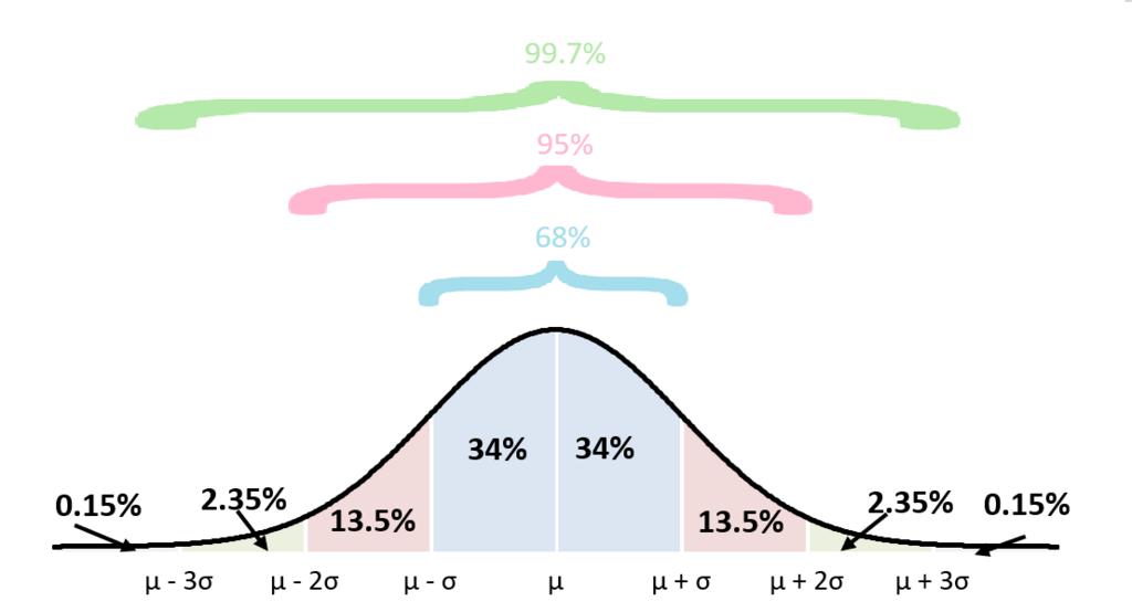
The power of the normal distribution comes from its predictability. For any normal distribution, we know that about 68% of the data falls within one standard deviation of the mean, 95% within two, and 99.7% within three. This is called the Empirical Rule.

But what if we want to compare values from two different normal distributions, like SAT scores and ACT scores? We need a universal standard. That's where the Z-score comes in. It re-scales any value from a normal distribution into the number of standard deviations it is away from the mean.

A positive Z-score means the value is above the mean, while a negative Z-score means it's below. By converting values to Z-scores, we can compare them on a common scale, the standard normal distribution, which has a mean of 0 and a standard deviation of 1.

Not all data is continuous like height or weight. Sometimes we're interested in counting things, which involves discrete probability distributions. Two of the most important are the Binomial and Poisson distributions.

The Binomial distribution models the number of successes in a fixed number of independent trials, where each trial has only two possible outcomes. Think of flipping a coin 10 times and counting the number of heads, or testing 100 products and counting how many are defective. The key conditions are a fixed number of trials ($n$), and a constant probability of success ($p$) for each trial.

The Poisson distribution is a bit different. It models the number of times an event occurs within a specified interval of time or space. For example, you could use it to predict the number of emails you'll receive in an hour, the number of customers arriving at a store in a day, or the number of typos on a page.

The main requirement is that these events happen with a known average rate and are independent of the time since the last event. It's especially useful for modeling rare events.

So far, we've discussed distributions for populations. But we almost never have data for an entire population. We work with samples. How can we use a sample to make conclusions about the whole population? This is the core question of inferential statistics, and the answer lies in the Central Limit Theorem (CLT).

The CLT is one of the most stunning ideas in statistics. It states that if you take sufficiently large random samples from a population, the distribution of the sample means will be approximately normal, regardless of the population's original distribution. This holds true whether the population is skewed, uniform, or bimodal.

This is incredibly powerful. It means we can use the properties of the normal distribution to analyze sample means, even if we know nothing about the shape of the population's distribution. This theorem is the bridge that allows us to move from describing our sample to making inferences about the population.

This leads to a crucial distinction: Standard Deviation vs. Standard Error The standard deviation measures the variability within a single sample. The standard error, on the other hand, is the standard deviation of the sampling distribution of the mean. It measures how much sample means are expected to vary from one another if you were to take repeated samples from the same population. A smaller standard error means your sample mean is likely to be closer to the true population mean.

Understanding which distribution fits your data is the first step toward choosing the right statistical test. These models provide the foundation for making predictions, testing hypotheses, and drawing meaningful conclusions from data.