You're likely familiar with linear equations like $y = 2x + 1$. When you graph them, you get a straight line. Every point on that line is a solution to the equation. But what if the relationship isn't so exact? What if you have a budget, and you can spend up to a certain amount, but not necessarily the exact amount?

This is where linear inequalities come in. They use symbols like $<$, $>$, $≤$, and $≥$ instead of a simple equals sign. For example, $y ≤ 2x + 1$ means that any point $(x, y)$ that satisfies this condition is a solution. This includes not just the points on the line $y = 2x + 1$, but all the points below it as well. Graphically, this creates a whole region of solutions.

To figure out which side of the line to shade, pick a test point that isn't on the line. The origin, (0, 0), is usually the easiest. Let's test it in $y ≤ 2x + 1$. Plugging in the values gives us $0 ≤ 2(0) + 1$, which simplifies to $0 ≤ 1$. Since this is true, we shade the side of the line that contains the origin. If it were false, we'd shade the other side.

Real-world problems rarely have just one constraint. A business might have a budget constraint and a production time constraint. A diet might have a calorie limit and a minimum protein requirement. When you have multiple inequalities that must be satisfied simultaneously, you have a system of linear inequalities.

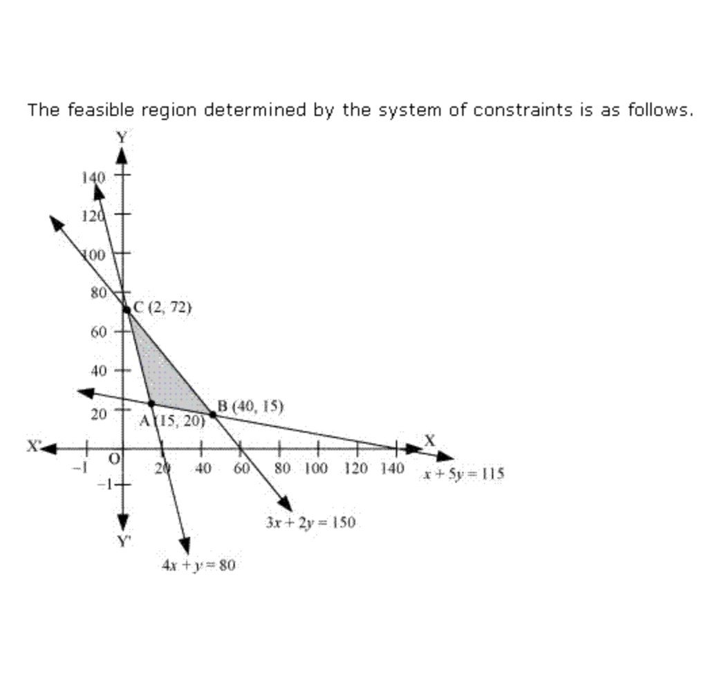
The solution to a system isn't a single point or a single region. It's the area where all the individual solution regions overlap. This overlapping area is called the feasible region. Any point within this region is a valid solution that satisfies every single inequality in the system. Points outside this region violate at least one of the constraints.

In the graph above, the solution to the system is the area where the blue and red shading overlap, creating the purple feasible region. Any point in this purple zone works for both inequalities.

The vertices of the feasible region are called corner points. These points are significant because they represent the extreme possibilities of the system. In optimization problems, like finding the maximum profit or minimum cost, the optimal solution almost always occurs at one of these corner points.

To find a corner point, you treat the two boundary lines that create it as a system of equations and solve for their intersection. For example, to find the intersection of $y = -x + 4$ and $y = 2x - 2$, you can set the expressions for $y$ equal to each other:

Once you have the x-coordinate, plug it back into either of the original equations to find the y-coordinate. Using $y = -x + 4$, we get $y = -(2) + 4 = 2$. So, the corner point is (2, 2). You would repeat this process for every pair of lines that intersect to form a vertex of your feasible region.

The real power of these systems is in modeling real-world constraints. Let's say a bakery makes cakes and pies. A cake ($c$) takes 2 hours of labor and a pie ($p$) takes 1 hour. The bakery has a maximum of 40 labor hours available per day. This gives us our first inequality:

$2c + p ≤ 40$

Additionally, the oven can bake a maximum of 30 items total per day. This gives us a second constraint:

$c + p ≤ 30$

Finally, it's impossible to make a negative number of cakes or pies, so we have two more common-sense constraints:

$c ≥ 0$ $p ≥ 0$

Graphing this system of four inequalities would give us a feasible region representing all possible combinations of cakes and pies the bakery can produce given its constraints.

If the bakery makes a profit of $25 per cake and $15 per pie, the total profit can be represented by the equation $P = 25c + 15p$. By testing the corner points of the feasible region in this profit equation, the bakery owner can find the exact combination of cakes and pies that maximizes their profit. This powerful application of linear inequalities is known as linear programming.