You've mastered the basics of voltage, current, and resistance. Now it's time to analyze circuits like a professional. When circuits get complex, with multiple power sources and interconnected branches, simple series and parallel rules are not enough. We need more powerful, systematic methods.

The first of these is Nodal Analysis. Instead of tracking currents through loops, we focus on the voltage at each critical connection point, or node. By applying Kirchhoff’s Current Law (KCL) at each node, we can build a set of equations that solves the entire circuit at once.

KCL states that the sum of currents entering a node must equal the sum of currents leaving it. Think of it like water pipes meeting at a junction; what flows in must flow out. In Nodal Analysis, we express each of these currents in terms of the node voltages using Ohm's Law. For any resistor $R$ between two nodes, A and B, the current flowing from A to B is $(V_A - V_B) / R$.

Let's work through an example. Consider a circuit with two unknown node voltages, $V_1$ and $V_2$, and a reference node (ground, 0V). By applying KCL at each unknown node, we create a system of linear equations. For a given circuit, the equation for Node 1 might look something like this:

We would write a similar equation for Node 2. With two equations and two unknowns ($V_1$ and $V_2$), we can solve for the voltages. This method scales beautifully to much larger networks and is the basis for most circuit simulation software.

What if you only care about what's happening at one specific part of a complex circuit, like the voltage across a single "load" resistor? Analyzing the entire network is overkill. This is where Thévenin’s Theorem becomes incredibly useful. It states that any linear electrical network with two terminals can be replaced by a single voltage source in series with a single resistor.

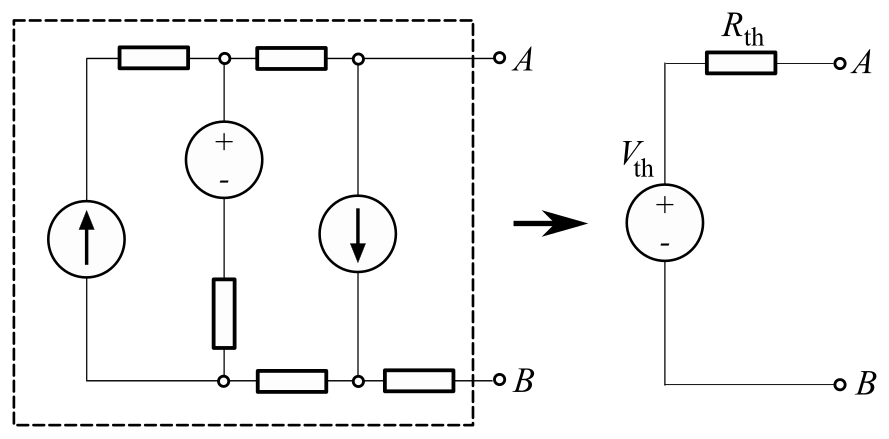
This simplified circuit is called the Thévenin equivalent. It consists of two parts:

1. Thévenin Voltage ($V_{th}$): The open-circuit voltage across the two terminals. You find it by removing the load component and measuring (or calculating) the voltage at those points.
2. Thévenin Resistance ($R_{th}$): The equivalent resistance of the network looking back into the terminals, with all independent sources zeroed out (voltage sources become short circuits, current sources become open circuits).

Once you have $V_{th}$ and $R_{th}$, you can easily calculate the voltage and current for any load resistor you connect.

This technique is vital for practical design, especially in load matching for maximum power transfer. Maximum power is delivered to a load when its resistance equals the Thévenin resistance of the source circuit ($R_L = R_{th}$). This principle is fundamental in everything from audio amplifier design to radio antenna systems.

Let's find the Thévenin equivalent for the circuit pictured below. We want to simplify the circuit connected to terminals A and B.

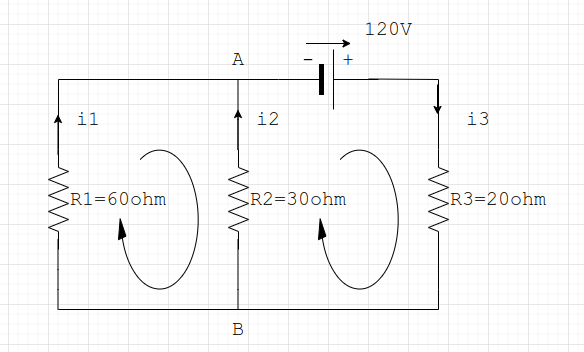
Step 1: Find $V_{th}$ We remove any load and find the voltage between A and B ($V_{AB}$). Since there's no load, no current flows through R3 (the 20Ω resistor). This means there's no voltage drop across it, so $V_{AB}$ is the same as the voltage across R2 (the 30Ω resistor). The 120V source is applied across R1 (60Ω) and R2 (30Ω) in series. We can use the voltage divider rule:

Step 2: Find $R_{th}$ Now, we zero out the 120V source by replacing it with a short circuit (a wire). Looking back into terminals A and B, we see R3 in series with the parallel combination of R1 and R2.

With this simple equivalent circuit, we can predict the behavior for any load connected to A and B instantly. For instance, if we connect a 10Ω load, the current would be $I = V_{th} / (R_{th} + R_L) = 40V / (40\Omega + 10\Omega) = 0.8A$.

Time to test your understanding.

Nodal and Thévenin analysis are fundamental tools. Mastering them allows you to deconstruct complex systems into manageable parts, a skill essential for effective circuit design and troubleshooting.