Every measurement in physics comes with an uncertainty. It's not a mistake, but a reflection of the limits of our instruments and methods. We need to quantify this uncertainty. The simplest form is the absolute uncertainty (${\Delta}x$), which has the same units as the measurement itself. For example, a length might be recorded as $5.2 \pm 0.1$ cm, where $0.1$ cm is the absolute uncertainty.

To compare the significance of uncertainties, we often use fractional or percentage forms. The fractional uncertainty is the absolute uncertainty divided by the measurement. The percentage uncertainty is just the fractional uncertainty multiplied by 100.

When you use uncertain measurements in calculations, the uncertainty carries through, or propagates, to the final result. The rules for this depend on the mathematical operation.

For multiplication, division, or powers, the process is different. You must work with fractional or percentage uncertainties.

When raising a value to a power, you multiply the fractional uncertainty by that power.

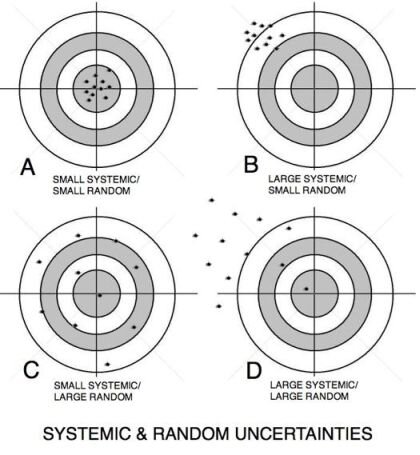
Experimental errors fall into two main categories. Random errors are unpredictable fluctuations in measurements. Taking multiple readings and averaging them can reduce the effect of random errors. They affect the precision of your results.

In contrast, systematic errors consistently shift measurements in a single direction. For example, a miscalibrated scale that always reads 5 grams too high introduces a systematic error. Averaging multiple readings won't fix this; it affects the accuracy of your results.

In graphs, we represent these uncertainties using error bars. An error bar is a line through a data point, parallel to an axis, that shows the uncertainty in that quantity. If you have uncertainties in both x and y values, your data point will have a cross shape.

The uncertainty in the gradient of a graph is a common requirement in IB Physics. To find it, you draw a line of best fit that passes as close as possible to all data points. Then, you draw two lines of 'worst fit'. These are the lines with the maximum and minimum possible gradients that still pass through the error bars of all data points. The uncertainty in the gradient is then half the difference between the maximum and minimum gradients.

Many quantities in physics, like force and velocity, are vectors. They have both magnitude and direction. To perform calculations, we often need to break a vector down into components that lie along the x and y axes. This process is called vector resolution.

Using trigonometry, we can find the magnitudes of these components. If ${\theta}$ is the angle the vector makes with the x-axis:

• The x-component is $V_x = V \cos{\theta}$
• The y-component is $V_y = V \sin{\theta}$

To add two or more vectors, we first resolve each one into its x and y components. Then, we add all the x-components together to get a total x-component, and do the same for the y-components. Finally, we use the Pythagorean theorem and trigonometry to combine these total components back into a single resultant vector.

Many relationships in physics are not linear. For example, the period of a pendulum relates to the square root of its length. Graphing this directly produces a curve, from which it's difficult to determine physical constants like the acceleration due to gravity ($g$).

A powerful technique is to manipulate the equation to create a linear relationship, $y = mx + c$. This is called linearization

Consider the equation for the period of a pendulum, $T = 2\pi\sqrt{\frac{L}{g}}$. To linearize it, we can square both sides:

If we now plot $T^2$ on the y-axis and $L$ on the x-axis, the equation is in the form $y = mx + c$. Here, $y = T^2$, $x = L$, the y-intercept $c = 0$, and the gradient $m = \frac{4\pi^2}{g}$. By calculating the gradient from our graph, we can rearrange the formula to solve for $g$.

Mastering these skills in handling uncertainties, vectors, and data linearization is fundamental for success in any experimental physics investigation.