Imagine a weather map, but instead of showing just temperatures, it shows wind. At every single point on the map, there's an arrow indicating the wind's speed and direction. That's a vector field. It’s a space where every point has a vector attached to it.

In two dimensions, a vector field is a function $\vec{F}$ that assigns a vector $\langle P(x,y), Q(x,y) \rangle$ to each point $(x,y)$. In three dimensions, it assigns a vector $\langle P(x,y,z), Q(x,y,z), R(x,y,z) \rangle$ to each point $(x,y,z)$. These fields can represent forces like gravity or magnetism, or the flow of a fluid like water or air.

Now that we have a field, let's travel through it. A line integral calculates the total effect of a vector field along a given path. Think about walking through a windy city. If the wind is at your back, it helps you along. If it’s in your face, it pushes against you. The line integral adds up all that help and hindrance over your entire journey.

We write the line integral of a vector field $\vec{F}$ along a curve $C$ like this:

Here, $d\vec{r}$ is a tiny vector pointing along the path. The dot product, $\vec{F} \cdot d\vec{r}$, isolates the part of the field vector $\vec{F}$ that points in the same direction as your path. If the field and path are aligned, the contribution is positive. If they are opposed, it's negative. If they're perpendicular, the contribution is zero.

To solve this, we parameterize the curve $C$ with a function $\vec{r}(t) = \langle x(t), y(t) \rangle$ for $a \le t \le b$. Then, the integral becomes a standard single-variable integral:

What if we want to measure how much of something is flowing through a surface, not just along a path? For that, we use a surface integral. Imagine holding a net in a river. A surface integral would calculate the total volume of water passing through your net per second. This is also called flux.

To calculate flux, we need to know the orientation of the surface at every point. This is given by a unit normal vector, $\hat{n}$, which is a vector of length one that is perpendicular to the surface.

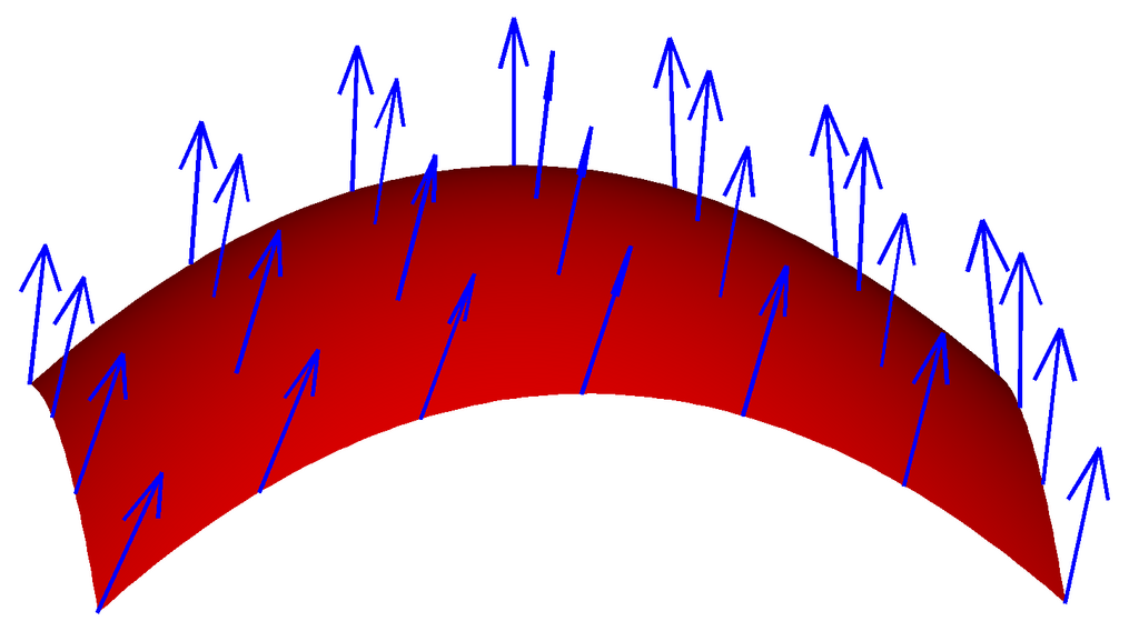
The surface integral of a vector field $\vec{F}$ over a surface $S$ is written as:

The dot product $\vec{F} \cdot \hat{n}$ isolates the component of the vector field that is perpendicular to the surface. If the field passes straight through the surface, the flux is high. If it runs parallel to the surface, the flux is zero because nothing is actually crossing it.

Two key operations in vector calculus, divergence and curl, help us understand the behavior of a vector field at a single point. They use the del operator, $\nabla$, which in Cartesian coordinates is:

Divergence tells us if a point is a source or a sink. A positive divergence means the field is expanding or flowing away from the point (a source). A negative divergence means the field is contracting or flowing into the point (a sink). Zero divergence means the flow in equals the flow out, like water in an incompressible fluid. It's calculated with a dot product:

Curl measures the microscopic rotation of the field at a point. Imagine placing a tiny paddlewheel in a flowing river. If the river's current makes the paddlewheel spin, the field has a curl at that point. The curl is a vector: its direction is the axis of rotation (found using the right-hand rule), and its magnitude is the speed of rotation. It's calculated with a cross product:

These concepts are the building blocks for the major theorems of vector calculus. Understanding them is key to unlocking a deeper view of how fields behave.