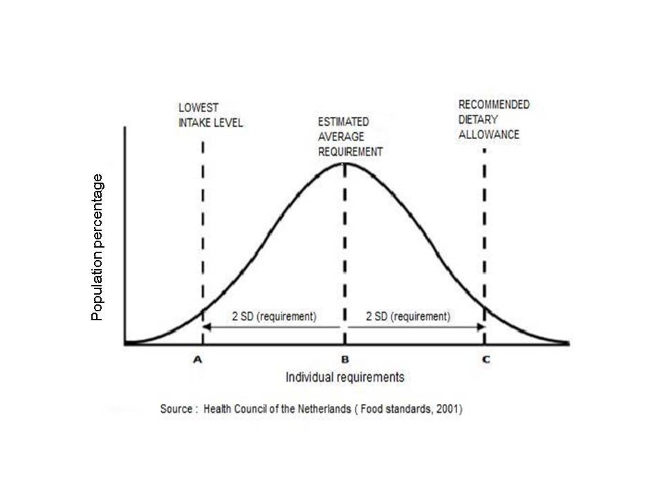
You're likely familiar with the classic bell curve, also known as the Gaussian or normal distribution. It's a way to describe the probability of a single random variable, like the height of a person or the outcome of a dice roll. The curve is centered on the most likely value, its mean, and its spread is determined by its variance.

What if we have more than one random variable? If we have a collection of random variables, say $X_1, X_2, ..., X_n$, we can describe their collective behavior using a multivariate normal distribution. Instead of a single mean and variance, we have a mean vector, which tells us the average value for each variable, and a covariance matrix, which tells us how each variable relates to every other variable. A positive covariance means they tend to increase together, while a negative covariance means one tends to go up when the other goes down.

Now, let's take a leap. Imagine you don't just have a few random variables, but an infinite number of them. Think of a function, $f(x)$. For every single input value $x$, the output $f(x)$ is a random variable. This infinite collection of random variables is what we call a Gaussian Process.

This might sound abstract, but the core idea is simple. A normal distribution describes the probability of a single value. A multivariate normal distribution describes the probability of a vector of values. A Gaussian Process describes the probability of an entire function.

Just as a multivariate normal distribution is defined by a mean vector and a covariance matrix, a Gaussian Process is defined by a mean function and a covariance function. These two functions tell us everything we need to know about the distribution over functions.

The mean function, written as $m(x)$, represents our prior belief about the function's shape before we see any data. It's the 'default' function. Often, for simplicity, the mean function is set to zero, assuming that, on average, the function's output will be zero everywhere. This is like saying we have no initial bias about where the function will be.

The covariance function, or kernel, $k(x, x')$, is where the real magic happens. It takes two input points, $x$ and $x'$, and tells us how similar the function's outputs, $f(x)$ and $f(x')$, are expected to be. If the covariance is high, the outputs will be strongly correlated. If it's low, they'll be nearly independent.

This function is crucial because it defines the properties of the functions in our distribution. A common choice for the covariance function might state that points close to each other should have similar values. This leads to smooth functions. Different covariance functions can produce functions that are rough, periodic, or have other interesting characteristics.

So, a Gaussian Process is a powerful generalization. It takes the familiar concept of a Gaussian distribution over a single number and extends it to an entire function. By specifying a mean function (our best guess) and a covariance function (how we expect the function to behave), we define a probability distribution over an infinite number of possible functions.

This provides a flexible and principled way to think about uncertainty in functions. Instead of committing to one specific function, we can consider a whole space of them, each with a certain probability. This is a foundational concept for many advanced machine learning models.