In linear algebra, we often think in terms of discrete transformations. A matrix acts on a vector and produces a new vector—a single, static snapshot of a change. But the world isn't a series of snapshots; it's a continuous flow. Systems evolve smoothly over time, whether it's the temperature of a cooling object, the position of a satellite, or the hidden state of a deep learning model.

To capture this continuous motion, we shift our perspective from transformations to dynamics. We represent the state of a system as a vector, $\mathbf{z}(t)$, which changes over time. The crucial question is not just where the state is, but how fast it's changing and in what direction. This is the domain of ordinary differential equations (ODEs), which describe the instantaneous rate of change of a state vector.

This single equation is the key to modelling continuous-time systems. The function $f$ acts as the universal rulebook, defining the dynamics at every possible state.

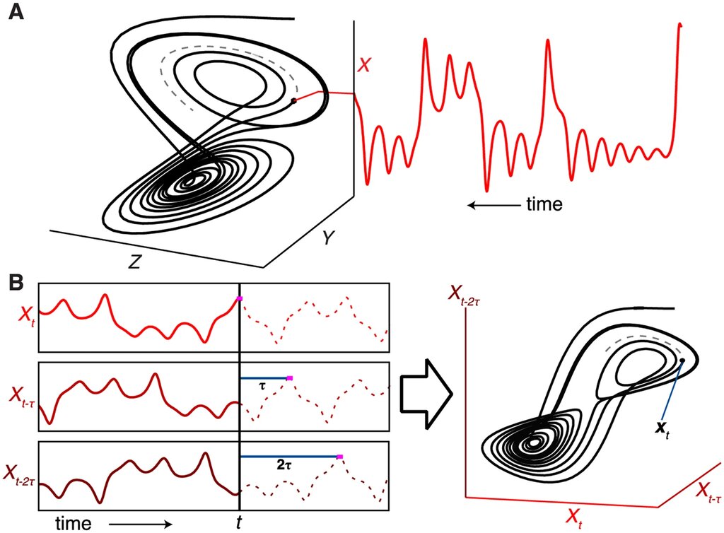
To understand a system's behaviour, we can visualise its dynamics in phase space. This is an abstract space where each axis corresponds to a component of the state vector $\mathbf{z}$. A single point in phase space represents one complete state of the system at a moment in time. As the system evolves, this point traces a path, or trajectory.

The function $f$ from our ODE defines a vector field across this phase space. At every point, the vector field assigns a vector that points in the direction of the state's instantaneous change, with its length representing the speed of that change. You can imagine it as a map of currents in a river. A leaf dropped anywhere in the river will follow a trajectory dictated by these currents.

Analysing this vector field allows us to understand the system's qualitative behaviour. We can identify equilibrium points where the vector field is zero ($rac{d\textbf{z}}{dt}=0$), meaning the system is at rest. Linear stability analysis helps us determine if these points are stable (nearby trajectories flow towards them) or unstable (nearby trajectories flow away). This is critical for predicting whether a system will return to a set point after a disturbance or spiral out of control.

What happens when we don't know the exact function $f$ that governs the system? This is a common problem in biology, economics, and physics, where we can observe a system's behaviour but don't have a perfect first-principles model. We have the data—the trajectories—but not the underlying vector field.

This is where a powerful idea emerges: we can use a neural network to learn the function $f$. This is the core concept behind Neural Ordinary Differential Equations (Neural ODEs). Instead of having discrete layers that perform fixed transformations, a Neural ODE uses a single neural network to represent the continuous dynamics of its hidden state.

The network takes the current state $\mathbf{z}(t)$ as input and outputs the derivative rac{d\mathbf{z}(t)}{dt}. To find the state at some future time $T$, we don't pass it through more layers. Instead, we give the network our starting state $\mathbf{z}(0)$ and ask an ODE solver to integrate the dynamics forward in time from $t=0$ to $t=T$.

This approach has significant advantages. Since the model is continuous, it can naturally handle data that arrives at irregular time intervals. It's also often more memory-efficient during training. Instead of storing the activations of every layer for backpropagation, we can use a clever technique called the adjoint sensitivity method to compute gradients.

By learning the underlying differential equations from data, AI agents can build more robust and flexible world models. They can predict the evolution of physical systems, understand complex time-series data, and operate in environments where information arrives asynchronously, moving AI from static snapshots to a true understanding of flow.