Finite Element Method in Python
Introduction to Partial Differential Equations
Equations in Multiple Dimensions
So far, we've dealt with changes happening along a single track. A car's speed changes over time. A population grows over time. These are described by ordinary differential equations (ODEs), which track a function of a single variable.
But the world isn't so simple. The temperature of a metal bar isn't the same everywhere along its length. It also changes over time as it heats up or cools down. The temperature, , is a function of both position, , and time, . It's written as .
To describe how things like this change, we need equations that can handle multiple variables at once. These are called partial differential equations, or PDEs. They use partial derivatives, like (how temperature changes with time at a fixed spot) and (how temperature changes along the bar at a fixed moment), to describe the full picture.
Partial Differential Equation
noun
An equation involving an unknown function of two or more independent variables and its partial derivatives.
PDEs are the language physicists and engineers use to model everything from the ripple of a pond to the flow of air over a wing. They don't just solve for a number; they solve for a function that describes a whole system—a temperature map, a pressure field, or the shape of a vibrating guitar string.
Three Flavors of Change
PDEs aren't all the same. They fall into three main categories based on the kind of physical phenomena they describe: parabolic, hyperbolic, and elliptic. These aren't just arbitrary labels; they tell us about the nature of the information flow in the system.
Think of it this way:
- Parabolic equations describe spreading or diffusion.
- Hyperbolic equations describe waves and propagation.
- Elliptic equations describe steady states or equilibrium.
Let's look at the most famous example from each category.
Spreading and Smoothing
Imagine touching a hot poker to one end of a cold metal rod. Heat doesn't instantly warm the whole rod. It diffuses from the hot end to the cold end, gradually smoothing out the temperature differences. This process is governed by a parabolic PDE called the heat equation.
It tells us that the rate of temperature change over time at any point is proportional to the curvature of the temperature profile at that point. A sharp, pointy temperature spike (high curvature) will smooth out quickly, while a gentle slope changes more slowly.

In one dimension (along the rod), the heat equation looks like this:
The key feature of parabolic equations is that a disturbance at any single point is instantly felt, however faintly, everywhere else in the domain. The information spreads infinitely fast but loses its strength over distance. It's a process of smoothing and reaching a uniform state.
Waves and Ripples
Now, think about plucking a guitar string. The disturbance you create doesn't just diffuse—it travels. A wave moves along the string at a finite speed. This is the world of hyperbolic PDEs, and the classic example is the wave equation.
Unlike the heat equation, where information spreads out everywhere at once, the wave equation confines information. A pluck at one point doesn't affect a distant point until the wave has had time to travel there. This property, a finite speed of propagation, is the hallmark of hyperbolic systems.
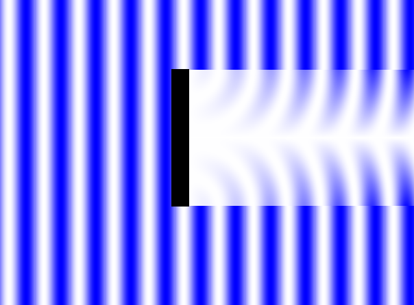
The wave equation relates the acceleration of a point on the string to the tension, or curvature, at that point.
This equation doesn't just describe guitar strings; it's fundamental to sound waves, light waves, and ripples in a pond.
Equilibrium and Balance
Finally, let's consider a situation that has settled down. Imagine a thin metal plate where the edges are held at fixed temperatures—maybe one edge is on ice and the opposite edge is over a flame. After some time, the temperature inside the plate will stop changing. It reaches a steady state, or equilibrium. This final temperature map is described by an elliptic PDE, Laplace's equation.
Laplace's equation states that the temperature at any point is the average of the temperatures of the points surrounding it. There are no bumps or dips; the temperature distribution is as smooth as it can possibly be, given the conditions at the boundaries. Unlike the other two types, there is no time variable. Elliptic equations describe systems in balance.
Because the solution at any point depends on the boundary values everywhere, a change in the boundary at one location immediately affects the solution everywhere else. Laplace's equation is also used in electrostatics to find electric potential and in fluid mechanics to model certain types of flow.
| Category | Key Idea | Classic Example | Physical Meaning |
|---|---|---|---|
| Parabolic | Diffusion | Heat Equation | Systems that smooth out over time. |
| Hyperbolic | Propagation | Wave Equation | Information travels at a finite speed. |
| Elliptic | Equilibrium | Laplace's Equation | Steady-state systems in balance. |
Understanding these three types of PDEs is the first step toward modeling the complex, interconnected systems we see all around us.
Ready to check your understanding?
What is the primary distinction between an ordinary differential equation (ODE) and a partial differential equation (PDE)?
A physicist is modeling how a drop of dye spreads out in a still tank of water over time. The concentration of the dye is a function of both position and time. Which category of PDE best describes this diffusion process?